Lecture notes on stability in the dynamics and Euler's method
This semester, I had the opportunity to do 7 weeks of “interactive lectures” at QUT for MXB261 Modelling and Simulation Science, as well as one guest lecture on evolutionary game theory. In this blog post, I’ll talk about my experiences, share the first half of one of the lectures I gave, and provide the code, to generate the figures, in case any of that is useful to anyone.
The Unit Coordinator is transforming the MXB261 into a game theory unit, and the first 7 weeks were “old” material she will replace in the coming years. Students responded really well to the new game theory content, describing it in the survey as “fascinating” and “mind blowing”.
Nonetheless, the old material was also quite interesting; one student still wanted to “go down the ODE rabbit hole” after the exam. The unit had no maths prerequisites, so any second- or third-year student curious about modelling could join, and it offered a “taster” of different modelling techniques, including Monte Carlo simulation, Markov processes, and ODE models. The case studies were focused on ecological applications, and it attracted students from maths, data science, and environmental science. I think it was quite unique with its goal of broadening students’ knowledge rather than going deep on a particular topic, and I would have really enjoyed it as a second-year undergrad (I did environmental engineering). I hope that the students will draw on it later in their professional career; if they have a particular problem to solve, I hope they will remember which types of techniques can be used to solve it, and build from the basic principles they learned here to teach themselves the rest of what they need to know.
The interactive lectures were “hybrid” lectures with students attending both in-person and online. The first half was typically structured more like a traditional lecture but with active-learning opportunities. I would work through additional material and the self-study activity, but pepper it with Q&A and pair-and-share. The second half was space for students to ask questions and get help with their assignments.
One challenge was teaching to students from a range of backgrounds. Some students found the MATLAB coding trivial but were thrown by mathematical notation, while others felt at ease with the mathematics but struggled with coding. So before each interactive lecture, I would review the activity and workshops, watch the online recorded lecture, and think about my 2 imaginary students: one who is good at maths but struggles with coding, and another who is comfortable with coding but not with maths. What is the implicitly assumed knowledge they might not have? What would they find unfamiliar and difficult? That would guide my content for the interactive lecture.
Below, I will share the first half of one lecture I gave. For this lecture, I noticed that the online recordings assumed that students would be familiar with initial-value problems and stability. For example, the stability conditions were given without an explanation for why they were so. So my lecture introduces quiver plots as a visual tool for understanding ODEs, then uses them to build intuition for steady states and stability, before moving to cobweb plots to explain numerical stability in Euler’s method.
It took quite a while to prepare this lecture, so perhaps this will save someone some time. The full list of MATLAB scripts used to create the figures is available from this blog’s repository, and I’ll link them in context below. One thing I found really helpful was to plot a thin grey line where I intended to draw during the lecture. The lines aren’t visible on the slides below, but were visible on the tablet I used, and that’s much safer than trying to free-hand it.
Although it might embarrass me a little, I’ve decided not to edit out my verbal hiccups. The transcript is pretty much how Zoom transcribed it except I removed some exchanges I had with students, added ellipses and removed muttering when I pause to draw, and corrected some Zoom-transcription errors. I’ve benefitted from looking at the transcripts of others’ lectures and seeing those verbal imperfections. The transcript also helped me notice a few verbal tics I would like to correct. I have almost succeeded in removing “um” and “like” from my vocabulary, but it’s a journey. I think I could reduce the number of sentences I start with “So…”. The main thing I would like to correct is my use of gendered language (“you guys”). This is not a good habit, particularly when I’m teaching maths.
Lecture transcript
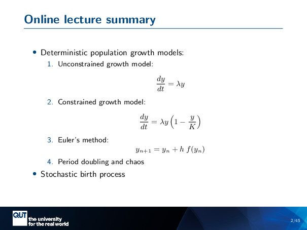
In your online lectures, you looked at deterministic population growth models, unconstrained growth, constrained growth. Then you looked at Euler’s method, and then a little bit of cool stuff with period doubling and chaos.
So, there’s no prerequisites for this course, and I know that, if that was the first time I’d seen this kind of thing, I would have been pretty bewildered. There’s certainly a lot of guidance on how to use Euler’s method and stuff like that, but learning is more than doing the activity, it’s understanding the meaning behind it. And so what I thought I’d do for this interactive lecture is introduce you to some visual tools to help you understand what’s really going on behind this maths.
So for those of you whose expertise is in coding and not so much in maths, I hope that this will be useful for you.
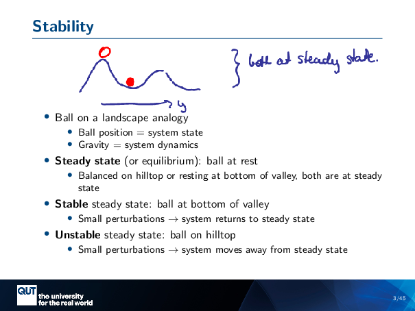
So it’s actually a legal requirement that any lecturer who talks about stability has to use the balls on a hill analogy. So, I’m going to do that. I’m going to consider two balls on a landscape. I’ll give this one an open circle, and this one a closed circle, and this is an analogy for the concept of steady state and stability.
In this, analogy, the ball position is like a system state. So we could imagine that the position here is Y, for instance, and gravity provides us our system dynamics. Now, these two balls, one perched on the hill and one in the valley, are both at steady state. So the meaning of steady state is that something doesn’t change with time. And both of these balls, as we watch them … they’re not moving.
But there is a sense that one of these balls is more stable than the other. Intuitively, a stable steady state would be the example of the ball at the bottom of the hill, that if we give it a small perturbation, if I pushed to the left, it would roll back to where it was. Whereas an unstable steady state is the ball at the top of the hill, where if I give it a bit of a push, then it’ll roll off down the hill and go away from that steady state that it started at.
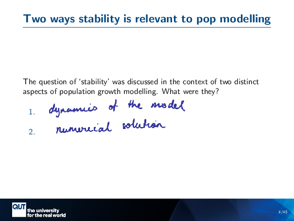
So in your online lectures, this question of stability was discussed in the context of two distinct aspects of the population growth modelling that you were looking at. What were those aspects? I’m going to get you to pair-and-share. And I am going to try something exciting and create a breakout room for the people online so that you can discuss as well, so hold on to your socks.
(Pair-and-share. No one was able to answer)
Fair enough. Okay, well, this is a great lecture, because I’m going to show you exactly what those two aspects of stability were. So I’ll just write them here… The two aspects of stability were the dynamics of the model itself. So the stability of the population. And the other aspect of stability was the stability of the numerical solution to the dynamics. So, in this lecture, I want to introduce some kind of visual tools to help us get a handle on these two aspects of stability.
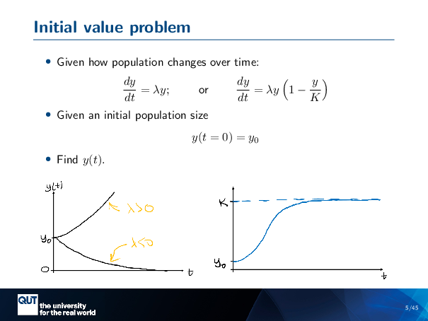
We’re given a class of problems called the initial value problem. And so the idea is that you’re given some kind of differential equation. These equations describe how the state variables change over time. So, in this case, the population size changes over time. And we’re interested in finding the trajectory of the population given the initial population size, given the initial values. And so, in this case, we start with Y at T equals 0 equals YO, and in the online slides, you are given these solutions to YT.
But I think maybe it might not have been so clear where these solutions came from. Certainly these examples have analytic solutions, but when we’re modelling– I mean, if we’ve got an analytic solution, we’re not going to break out the MATLAB, right? We just write it on a piece of paper. And so usually, when you’re using these sorts of techniques, you don’t have an analytic solution. And it’s not super obvious where these solutions came from.
So, what I want to do is first introduce you a tool called the quiver plot. And this is a visual tool for understanding how the system dynamics works.
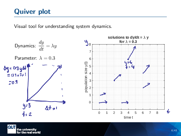
Figure scripts: plot_one_quiver.m
So, in this case, I’m going to look at the unconstrained growth, model. So dY dT equals lambda y, and I’ve just set lambda equal to 0.3. So the idea of the quiver plot is that we, say, start at a point, say y equals 3, T equals 2, What we’re going to do is we’re going to take a delta T. In this case, I’ll set delta T to 1. And then we calculate, with that delta T, what will be our delta Y? So, we calculate our delta Y, is equal to 0.3 Y delta T. And so that would be, in this case, 0.3 times 3 times 1, because I set this one to 1. And so that’s how we get the length of this arrow here.
And then we basically draw an arrow in space, like that, on our graph. So here was Y equals 3, T equals 2, so that’s that point. And so, if I move along in time by one step, then I go up by … sorry, I forgot to do the final calculation … 0.9. Then we move up by 0.9, so up to there, so we draw a little arrow like this.
And so we can do that at various points in the grid. For example, let’s start here with Y equals 6, T equals 4. So we’re gonna take a step of T equals 1, and so the height of Y will be, let’s see, 6 times 0.3 is 1.8, so we’ve got to go to there. So we draw an arrow like that.
And we can do this in every spot on our grid to get a kind of sense of the dynamics… This is an important one. When Y equals zero, always the change in Y will be equal to 0.
And so imagine that I did this for the entire space of Y versus T. And I end up with this plot, which is called the quiver plot.
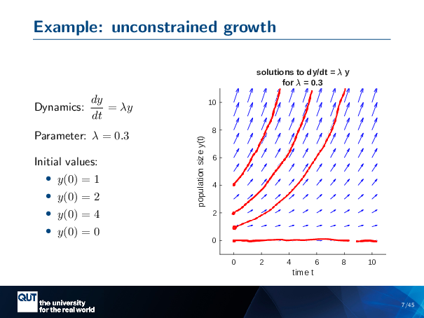
Figure scripts: plot_expon_growth.m
And this is fantastic, because this is DYDT equals lambda y. These little arrows are like a visual representation of the differential equation that you can see with your human eyeballs.
In addition, it has this very intuitive feeling about it, like there’s a flow of Y in time. And that intuition is correct. We can basically use that flow to understand where our solutions to DYDT equals lambda y goes from various initial values.
So let me be concrete about that. Let’s say I want to start at Y0 equals 1. So I put a little dot here. Now, you can see that there’s an arrow in that direction, and so I’m going to draw a line in that direction. This is Y changing with time. As Y gets larger, it gets entrained into these arrows that are headed more upwards. And so it increases … at an increasing rate … like this. And so that’s it, that’s one solution to the initial value problem, YO equals 1.
We can do another one. Let’s say we want to start at YO equals 2 … we catch our arrow, and we follow those arrows through time.
Here’s YO equals 4.
And of course, a pretty important one, Y equals zero … Our arrows are just going along like this, through time.
And so that’s how the initial value problem works, that dy dt gives us this … well, there’s an infinite number of arrows, but I can only draw so many. The initial value gives us where our solution starts, and the differential equation how we’re going to follow that flow through time.
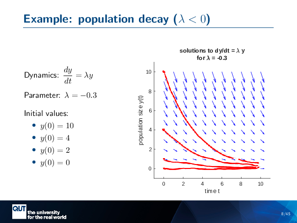
Figure scripts: plot_expon_decline.m
So that was the unconstrained growth model. Here’s another example with population decay. So this is the quiver plot, but it’s pointing in the other direction now, because our lambda is a negative number here. And we can do the same thing again.
So let’s start at YO equals 10, and we’re following our arrows down… And that’s one of our solutions to the problem.
If Y equals 4, start at 4, Following it down … And that’s another way that the population might change over time. Here’s another one. And if we have zero … then they will stay zero forever.
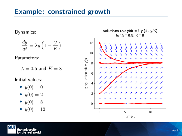
Figure scripts: plot_logistic.m
This one is the dynamics of the constrained growth, and it’s a bit more exciting because we’ve got arrows going in different directions, but the same principle applies. So we start at YO equals 0 … If we have no animals, there’ll be none forever.
Y equals 2 …
This is a special value: this is 8, the carrying capacity. And so if we’re at carrying capacity, we stay at carrying capacity forever.
And if we’re above it, well, that’s too many, so some … some animals are going to die… it’s the generations turn over, and we’ll go back down to carrying capacity.
So that’s where those lines came from in the online lectures. You can solve them analytically, but in the cases where you cannot, this is a kind of visual understanding of where the solution comes from.
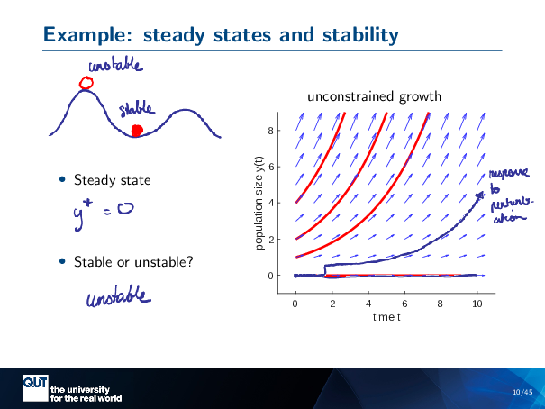
Figure scripts: plot_expon_growth_compact.m
So, remember, our analogy of the balls? We’ve got the unstable ball here … The stable ball here.
The first question we ask ourselves is, well, in the analogy, both of the balls were at steady state, because if we watch them through time, they don’t change.
And so, is there some point in this, in this flow, where if Y is at that value, it doesn’t change through time? And so, we’re looking at this, and … evidently, if we start at zero … we stay at zero forever. And so we will call this our steady state. Indicate it with a star … equals zero.
Now, the next question, is it stable or unstable?
So, when we’re thinking about our balls, if we give them a bit of a push, do they come back to where they were, or do they roll off to somewhere else?
So let’s give our steady state a bit of a push… And it gets entrained by an arrow that’s ever so slightly going upwards. And then it rolls away from y equals 0. So that means that Y star equals 0 is unstable.
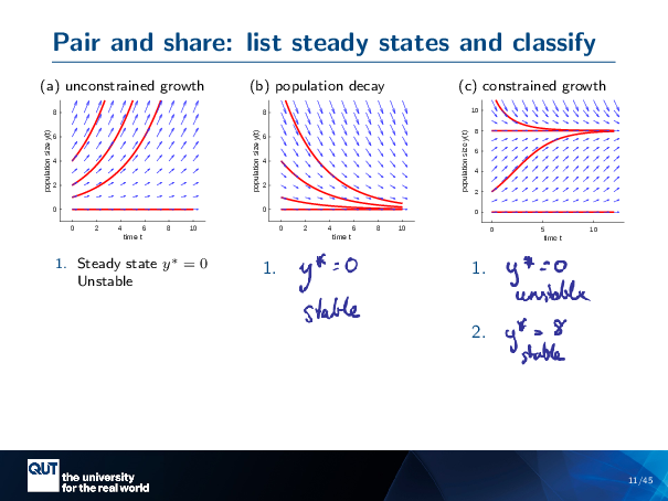
Figure scripts: plot_expon_growth_compact.m, plot_expon_decline_compact.m, plot_logistic_compact.m
So I just did the unconstrained growth example, and I think that, as a pair-and-share, you guys could do the other three cases.
So do the population decay and do the constrained growth, identify the steady states first, and then mark them unstable or stable. Alright, I’m gonna try this breakout rooms thing again.
(Pair-and-share)
Okay, yeah, so, so what did we conclude for the population decay one? What’s the steady state for that one? Plug it into the chat or shout out. Y is 0. Yeah, awesome, yes, exactly!
So in Y-Star, Equals zero, that’s our steady state. And is this one stable or unstable? Will be stable? Chat? You didn’t hear that answer, so have you guys got an answer to whether it’s stable or unstable? Stable, awesome, yeah! So you’ve got the idea that if you give this a bit of a push. Then it’s going to come back to where it was before.
Okay, now this one’s a bit more complicated. It’s got two steady states. Let’s just pick one. What’s one of the steady states? That’s the full answer from the chat! Real fast. Yes, excellent. So here’s a … steady state, Y star equals 0. And this one is unstable, because if we give it a bit of a push, it’ll get entrained into those, arrows and move away. And then there’s Y star equals H, which was our carrying capacity, and this one’s stable. And so you can see that if we push it up or down, it’s going to come back to where it was before.
Alright, so we’ve got our intuition nice and primed!
But we’re probably not going to be plotting quiver plots to understand the stability of our system. So, is there some kind of mathematical way that we can capture this intuition and do it with maths?
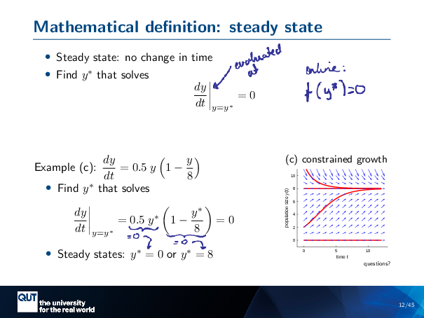
Figure scripts: plot_logistic_compact.m
So, steady state means that there’s no change in time. And so that means that we’re looking for a DYDT that stays zero for the, entire time.
So I’ve got a bit of new notation here that might be new to you. What this means is it’s “evaluated at”. So I’m going to calculate DYDT, but I’m going to evaluate it at the particular Y star that it will be equal to 0 at.
That was a bit of a clunky explanation. Your online lecturer uses FY star equals 0 instead… I find F not very descriptive, so I’m going to keep using this notation here.
So let me give you a concrete example. Here’s the constrained growth. There’s my DYDT. And so what I do is I substitute in everywhere where there’s a Y, I’m going to put in a Y star. And I’m going to make that equal to zero, and then I’m going to try to solve it.
What are the Y stars that make this equal to zero? So, we’ve got a product here, so that means that it can be zero if either this part is equal to zero, or that part is equal to zero. So this left-hand side, that’s equal to zero when y star itself is equal to zero, so that’s that solution there. And this right-hand side, well, that would be equal to 0 if Y star on 8 is equal to 1, which means that Y star is equal to 8, and so that’s… So that’s how we get our steady states mathematically.
Okay, so we’ve got our steady states. But how can we tell if they’re stable or unstable? We’ve been looking at the quiver plot so far, but is there some mathematical way to check if it’s stable or unstable as well?
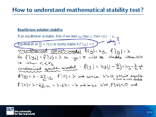
And so, in your online lectures, you’re given, in particular, this part here is the important bit. So apparently, if this derivative is less than zero, then it’s stable.
Okay, cool. So we could memorize that, but why is that the case? Like, can we get some intuition going for this?

Figure scripts: plot_expon_growth_compact.m, plot_expon_growth_dydt.m
So, to get the intuition for this, I’m going to do something, a little bit new. This is the plot that I had before. Here, DYDT versus Y. And so I’m looking at my unconstrained growth again.
And this is the line that I’m interested in plotting… DYDT versus Y.
When y equals 0, DYDT equals 0, so we’ll start here. And what’s an easy second point? When y equals 10, DYDT equals 3, so we’re going to that point there. So this is a straight line. So that’s our DYDT versus Y.
So now, what I’m going to do is I’m going to draw a cartoon of the dynamics on this axis here. And, this is something that’s commonly done in the literature, I’m going to use the same conventions as them.
So, what I’m going to do is, on this axis, on this line, I’m going to draw an arrow that goes in the positive direction, if there’s a positive change. If DYDT has, if Y has a positive change, or DYDT is positive. And I’m going to draw an arrow going in the negative direction, if it’s negative.
And I’m also going to identify the steady states by drawing an open circle … for our unstable states, and a closed circle … for our stable states. So it’s the same as the balls before. I planned ahead.
Alright, so how do we do this? So, I’m looking at DYDT, and I see that it’s positive, so I’m going to draw an arrow like this.
I could go a little bit further. I know that then when Y is quite large, the arrow is quite large. But then Y is small, the arrow is small. And indeed, DYDT here is high when it’s high and low when it’s low. So I could draw a … big arrow here, and a small arrow here, to kind of indicate that.
And so I know that the steady state is where Y equals 0, and at this point, I can actually just stop thinking and look at where the arrows are pointing. The arrows are pointing away from the steady state. So that means there’s an unstable steady state. So I’m going to put an open circle right here.
So this is my cartoon for the dynamics.
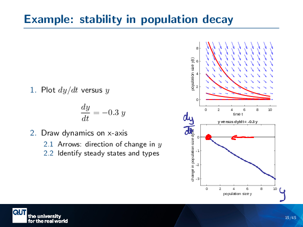
Figure scripts: plot_expon_decline_compact.m, plot_expon_decline_dydt.m
Do the same thing for the population decay. So, we’re going to draw a… DYDT on this axis, and Y on that axis. So when Y is 0, that equals 0. This time it’s a negative 3 with y equals 10. And I see that everywhere … this is negative, so I’m going to draw the negative arrow. And so the arrow is pointing towards my steady state, and so I’m going to put a stable steady state there.
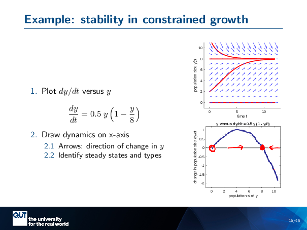
Figure scripts: plot_logistic_compact.m, plot_logistic_dydt.m
This is the fun one. So this, DYDT, it ends up being a bit of a curve … that starts here … and then goes down like this.
I think the purpose of all of these sorts of things is to not have to think too hard. So what have we got? We’ve got positive here … in here, it’s negative. And so immediately, I’ve got it: unstable steady-state, stable steady-state.
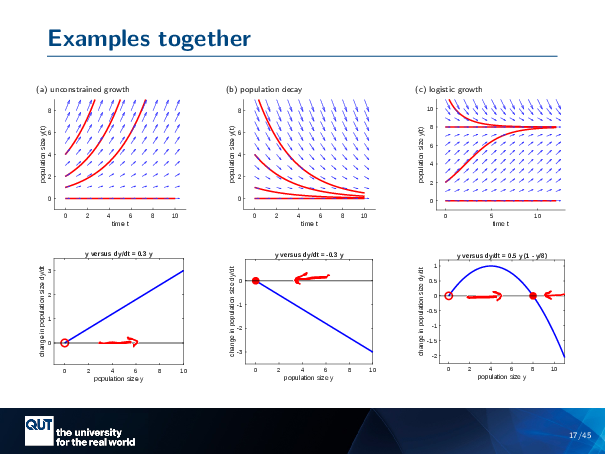
Figure scripts: plot_expon_growth_compact.m, plot_expon_decline_compact.m, plot_logistic_compact.m, plot_expon_growth_stability.m, plot_expon_decline_stability.m, plot_logistic_stability.m
Alright, so these are the examples together. This one had an arrow going that way, that one had an arrow going that way … this one has arrow going like this. And in fact, I could have drawn the arrows first, and then decided on the stability.
Are there any questions about that so far?
At this point, we’re just kind of creating a visual tool, and it’s going to hopefully get us towards the maths in a moment.
No questions from chat? Okay, we’ll keep going.
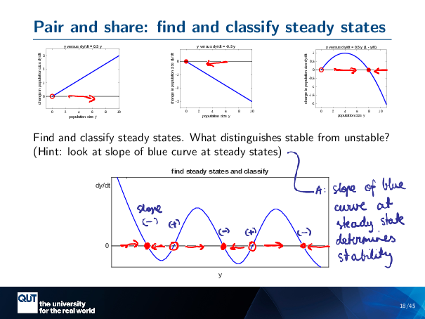
Figure scripts: plot_expon_growth_stability.m, plot_expon_decline_stability.m, plot_logistic_stability.m
Alright, so those were my examples that I just went through before. And so what I’m going to do is I’m going to get you to all pair and share. I’ve given you an arbitrary DYDT versus Y curve here, and I want you to do the same thing that I did before. Find out where the arrows point, and then find out where the steady and the stable and unstable steady states are. We’re gonna do the breakout rooms again. Getting good at this.
(Pair and share)
Alright, so .. help me out here while I do it. So, okay, let’s start at this point. Am I drawing a positive or negative arrow at that point? I hear a whisper of positive. Heading right, yes. Okay, and how about this one here, in between? Left! Alright, I think you guys get it. And so, this one’s positive because the curve is above, and it’s positive, and this one’s negative because it’s above it.
And so at this point, we don’t have to think anymore. This one’s stable, this one’s unstable, this one’s stable, this one’s unstable, this one’s stable.
Alright, now there was a second part: what is it that distinguishes the stable from the unstable steady states? With respect to the slope of the blue curve at those steady states? Did anyone notice a pattern?
Hmm. Over to under means stable, and under to over means unstable. Yep, definitely. So, yes. Over to under means stable. So, over to under.
What would the slope of that be? Would that be positive or negative? Yeah, you got it. It is, it’s negative. So this one’s got a negative slope. And this one’s got a positive slope.
I’m talking about the slope of the blue line, right? At this point, the blue line has a negative slope. At this point, it has a positive slope. At this point, it has a negative slope.
So it looks to us that the thing that distinguishes our stable from our unstable steady states is the slope of dydt with respect to Y.
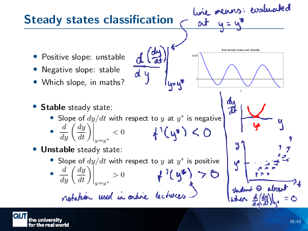
Okay, so let’s consolidate all that. When we’ve got a positive slope, it’s unstable. When we’ve got a negative slope, it’s stable. So how could we write this mathematically?
So, we’ve got DYDT on this axis, and Y on that axis. So, slope is d-something d-something, and it’s DY on the bottom because that’s the one that’s on our x-axis, as confusing as that is.
And what is it the slope of? Well, it’s the slope of DYDT. So this is the … this is the quantity that we’re using to determine whether our steady state is stable or unstable.
Now, this function will give us the value of that slope at every point. But we’re not interested in, like, the slope here, or here. We want it specifically at the steady states, right? So then we’re going to use our line notation to say we’re going to evaluate that … at Y equals Y star. So this is one of our Y stars, for instance. So this here … means evaluated here.
So I’ve written that out here, each of the cases. We’ve got a stable steady state when the slope of DYDT with respect to Y evaluated at Y star is negative. In your online lecture notes, they used a more abbreviated notation … like this … where it’s understood that F is DYDT, but I find that kind of counterintuitive. I like it to be more verbose, so I know what’s going on.
And likewise, if it’s an unstable steady state, well, we’re looking at that same quantity, but it has to be positive. And so, in your lecture notes, it looks like that. And so, you know what? Now you understand what that online lecture was saying.
(Student asks: What if the derivative is zero?)
You want to know about the equals zero case, don’t you? Okay, let’s do it. Alright, so let’s imagine… well, let’s look at an example. So, if we had … DYDT, and we had Y, in order to have it exactly zero, we’re going to need something like this … at our Y star, it has to be flat. And so one way we could do that is we could have it … looking like this. So what would that look like in our quiver plot? Let’s say that, I put my Y star here, and this is time. So now I’m doing Y versus T. So it means that as we’re approaching Y-STAR … our, our, … well, let’s see, they were, they were quite … and then they kind of went like this … and then they went like that, and then they went like that. But then they go positive again instead of going negative, and so they go up like that. So, if you imagine that one trajectory as a huge quiver plot — I’ll draw a better picture of this for the annotated notes — then that would be what you’re looking at, so it’s a point of inflection. … All of the examples you’ll be working through, it’s either positive or negative, so you don’t look at this kind of this in-between-y situation.
Are there any more questions about that? How about you, chat? I’m looking at the window. It’s all good. Alright.
Okay, so now we’ve got a mathematical way to do this, let’s do an example, a concrete example, so we can really solidify this.
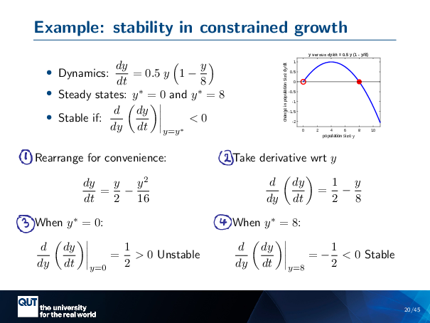
Figure scripts: plot_logistic_stability.m
So, this is our constrained growth again, because it’s my favourite. And we’ve got the dynamics here, and these steady states we found before. They were Y equals 0 and Y equals… Y star equals 8. And we knew from drawing our picture when it was unstable or stable, but let’s do it with maths to verify.
So, we want to look for, it’s stable if DDY of DYDT, evaluated at Y star is less than 0. So the first thing I do is, I just rearranged it, I expanded it out, because it’s easier to take the derivative then. So, I want to take the derivative of Y on 2, so that’s 1 on 2, so that’s that first term there. And this turns into 2Y on 16, which is Y on 8, so that’s there, and there’s your negative coming over. And so, at this step, now we need to — because we don’t want to know about the slope there, we want to know about it here and here, at each of the steady states — so we’re going to look at each of the steady states.
When Y star equals zero, what we do is we substitute Y equals 0 into this, so that would make this part 0, and that would leave a half, so that’s our half there. Half is greater than zero, so it’s unstable, which is something we verified before.
Now let’s think about when Y star equals 8. So if we put an 8 in here, that’s a 1, and a half minus 1 is a negative half, and so that’s that negative half there. Negative half is less than 0, and so it’s stable, and we knew that from before. Are there any questions about that?
Cool. So that was one aspect that stability that is important to us in population modelling, the stability of the dynamics of the model itself, of the population itself, at its different points in Y.
The second aspect is the stability of the numerical solution to the model. And so there’s similar concepts, but subtly different concepts here, and it can get a bit confusing.
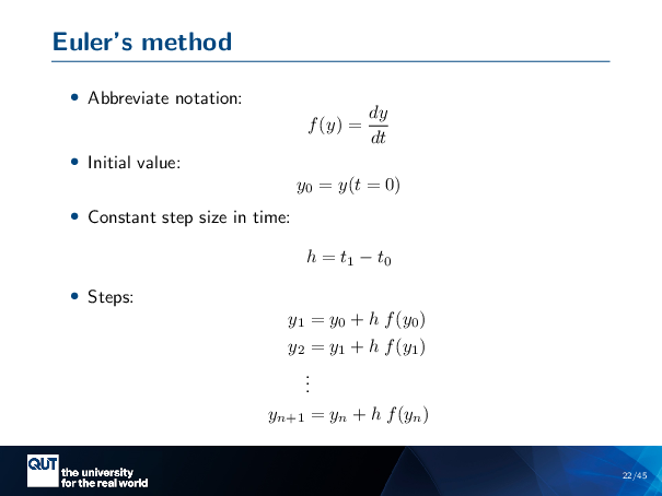
In your online lectures– I am going to abbreviate the notation now, I’m going to write F of Y for DYDT – and you would be given an initial value, YO, and you’re given a constant step size and time, which is H, and then you can just kind of churn through the maths. What you do is you get your YO … you put it into this equation and in here to calculate your Y1. And then you substitute your Y1 in to get your Y2, and yada yada yada. And it’s really boring. But what’s actually going on behind here? Something exciting.
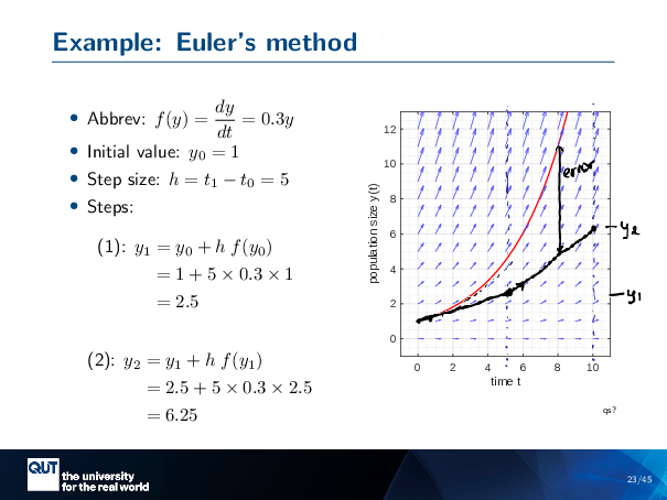
Figure scripts: plot_expon_growth_euler.m
Let’s take a concrete example, using, again, this awesome tool called Quiverplot. So … Here I am using my abbreviated notation for this particular example. I’m going to start at Y equals 1, and we know that our analytic solution here is this curve. So I’m going to take a step size of H equals 5. So what I’m saying is that I’m going to step forward in time by 5. So, just to make that … clear, I’m going to put a dotted line at the 5 … and at the 10 … That’s what we’re heading towards.
Alright, so you have seen examples of how to do this mathematically, here, we have the first two steps. So get Y0 equals 1 … we substitute it in, so there’s our 1. This here is our 5 from the H. 0.3 is that 0.3 up there. 1 is because we’re at H … YO equals 1 … and that equals 2.5. And then we can substitute that in to get the next one. So we put 2.5 in here and in here. This part here is the DYDT, and we get 6.25.
It doesn’t feel very meaningful. But we can understand what’s going on if we draw what the Euler method is doing visually.
So when we’re at YO, we’re starting here. And we’re going to take a step to calculate our Y1. What we’re doing is we’re catching this arrow that’s pointing in this direction. What we’re going to do is we’re going to say that’s the derivative of this function until we hit the wall at 5, so we’re going to project ourselves forward…. And here we are … that’s our Y1 at 2.5.
That’s what the Euler Method does. It takes the derivative at the point you started at, and steps forward in time using that derivative to get the next value.
At this point here, we’ve got an arrow that kind of points in that direction. And so we’re going to assume that that’s constant until our next point in time. And so we get to this point here … and so if I’ve drawn it well, that should be 6.25.
You can imagine that if I took more sensibly small steps, I would have tracked the value a little closer. But I took these big steps, because I wanted to show you the first issue with Euler’s method, which is that it’s not so great. So you can see here … Take the distance from, say, here to here … this is a lot of error. And you can imagine, as this red line goes up, the error’s just getting worse and worse. That’s also true if I’d have taken smaller step sizes, that error would be getting worse and worse, but it’s easier to draw them large.
So you might be thinking, well, maybe that’s just because this is, like, the exponential growth, and so maybe if you had some true … solution that sort of asymptotes that you would kind of … the solution that you’re finding with Euler’s method will get closer and closer to the true value. And that’s true, that is good intuition, and that is correct.
However, there’s other perverse things that can happen with the Euler’s method, even when you’ve got this asymptoting kind of situation. And so that brings us to the second aspect of stability, which is not the stability of the dynamics themselves, but the stability of the Euler method, whether it converges on the steady state of the dynamics or not.
So let me make that concrete.
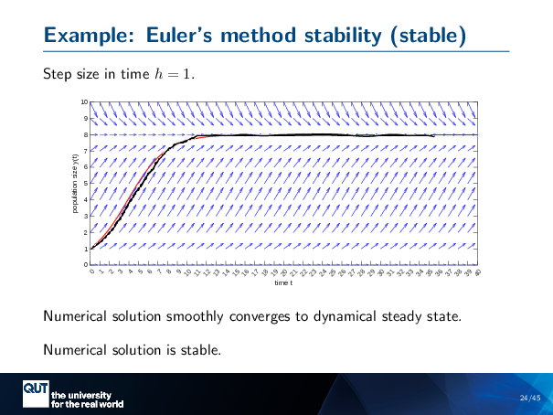
Figure scripts: plot_logistic_euler.m
So, here I’m taking really small step sizes … H equals 1 … And there’s my first step, my second step, my third step. The reason I’m able to do this is because I put a grey line in there to help myself later. And you can see it nicely converges to the dynamical, stable steady state. So the numerical solution is smoothly converging to the steady state, and here we would say that the numerical solution is stable.
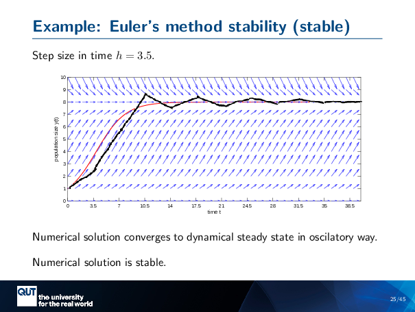
Figure scripts: plot_logistic_euler.m
Let’s take slightly bigger step sizes. I’m going to use a step size of 3.5 this time. So my first step takes me to here … My next step takes me to here … The next step takes me to here, oh, wow, I bumped over the steady-state. … then I bumped back … Boom, up, and down … But each bump, I’m getting closer and closer, until the bumps are kind of hard to see, and it basically looks like …
So, this numerical solution also converges to the dynamical steady state, but it does it in this oscillatory way. It goes above and below and above and below, switching, until … but it’s getting closer and closer. So we can say the numerical solution is also stable in this situation.
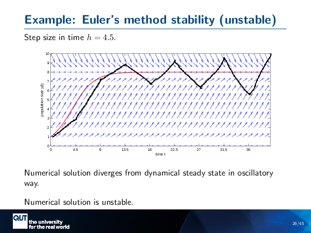
Figure scripts: plot_logistic_euler.m
Let’s make our step size even bigger. Alright, 4.5. So, take a step of 4.5, up to here … The next step gets me to here … So it’s oscillating like it did before…. Something bad is happening … Each time I oscillate, I catch one of those, those arrows that’s steep enough to send me further and further away. And so this oscillates and goes away in its oscillations from the steady state. And so this diverges from the dynamical steady state in an oscillatory way, and so we’d say that the numerical solution is unstable.
So note here, though, that the dynamics are stable. The dynamics of the population is stable. It’s the numerical solution that’s unstable. This is the two aspects I was talking about before, two aspects of stability that matter to us when we’re modelling, for instance, population growth.
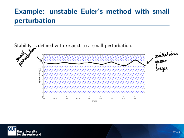
Figure scripts: plot_logistic_small_pert.m
Now, stability is usually defined in terms of the small perturbation. So we give our ball a tiny knock and see if it rolls down, right? So let’s, let’s look at stability with respect to a small perturbation.
Here we’re doing H equals 4.5 steps. So, imagine that we’re coming along just fine here … so our Euler’s method, when it’s on that 8, will stay at that 8, because it’s always changing by 0.
Now we perturb it a little bit, and we’ll have an oscillation…. And with each step, our bounce gets higher and higher … And so this one’s still diverging as well.
Before, I showed you us approaching the steady state, but really, we define stability with respect to a small perturbation near the steady state. You can see that, again, yes, it’s unstable, as we thought before.
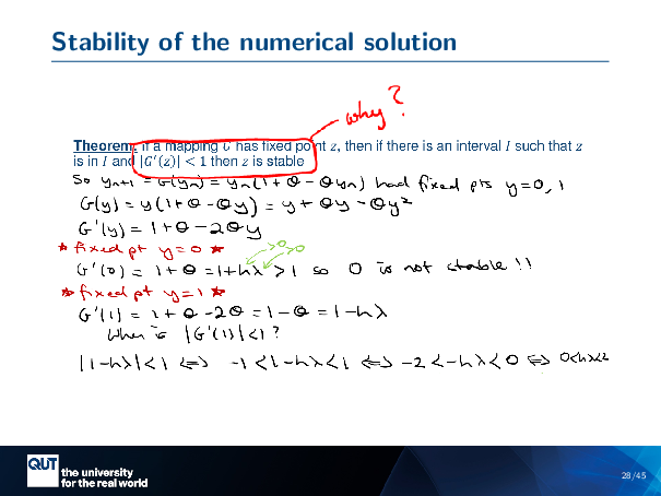
In your lecture notes, in your online lectures, there’s a slide about this, and it talks about a mapping, G, and if it has a fixed point, and the key quantity here is … if the absolute value of G-Z is less than 1, then Z is stable.
And so this is confusing, because we were talking about stability before, and we were looking for derivatve less than 0 and greater than 0, and now we’ve got an absolute value ..
What’s going on here? What is the meaning of what’s happening here?
I could leave you on a cliffhanger. I’ve got fair bit of content to get through. Do you guys want a 5-minute break, or do you want to push through? Short break. Short break, excellent idea.
(Break)
Alright, so where were we? So we’ve got this idea of stability of the numerical method. And we have an example of the Euler’s method being unstable with respect to a small perturbation. And so, in our online lectures, we were told that we’re to take some derivative, find its absolute value, see that it’s less than 1, and that means it’s stable.
And we’re like, okay, but why?
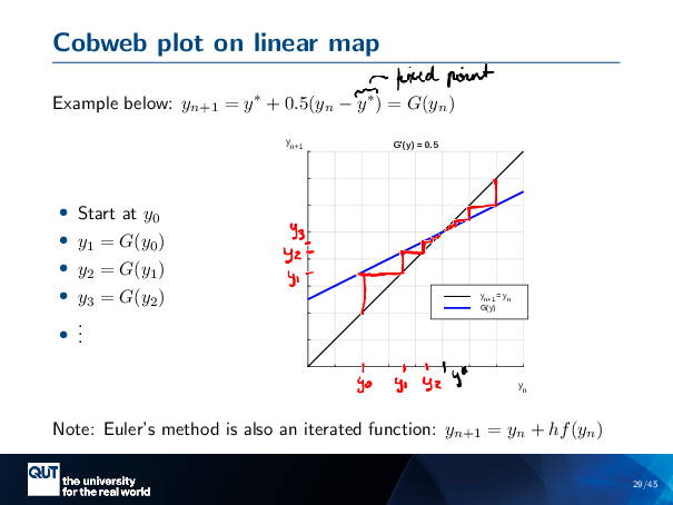
Figure scripts: plot_cobweb_stable.m
The second friend I’m going to introduce you to tonight is called the cobweb plot. This is another visual tool, a bit like the quiver plot I showed you before, and it’s used for understanding something called a linear map.
So, you’ve seen this kind of thing before, where you have some value at the next step, and it’s equal to some function of the value at the previous step. And here we’ve got some Y stars, and that happens to be the fixed point, so I might write that in there, actually … Fixed point. Which means that if we start at Y star, then Y… n plus 1 will equal Y, N will equal Y star. And this is our G that’s, defined in the online lectures.
So, how would we go about solving this kind of visually? What I’ve done here is I’ve plotted, the one-to-one line. And here I’ve got YN, our previous step, and YN plus 1, our next step. And this here is .. the function G, up the top there. This is our fixed point where the two lines meet.
And so, how would we do this mechanically? So we might start at some Y0 value. And then to get to Y1, we evaluate, G at Y0. And so, that corresponds … to this point here. And so visually, we might … just draw a line to indicate that, and that’s our Y1. So the next step in this process is that we take our Y1 value, and we substitute it into G again to get our Y2. And so, we need to find … set our YN equal to Y … Y1, we can actually kind of draw a line there, and you see where that touches the one-to-one point, is where our new Y1 is? We can do a step to our next Y2, so we’ve marked that here…. And then we’re going to substitute our Y2 into G to get our Y3 … Y2, you’re going to go up, and that gives us our Y3 ..
And so you can see that this, staircase thing that I’m drawing is basically keeping a track of our Y1, Y2, Y3, and so on, values, and … it staircases into this point.
We can do it from the other end, if we’ve started here. We would go … Well, the point of these is usually to stop thinking, so you go … Vert G … horizontal 1 … vert G … horizontal 1 … And so on. So it’s a visual representation of using this iterative map.
Are there any questions about what I’ve drawn there? Does that make sense? I’m not getting a yes or a no. Okay, so the reason that I’m showing you this … yes, okay, great, thank you. It sort of makes sense.
It seems a bit less useful than the quiver, yeah? That’s because I haven’t told you how it’s useful yet.
Alright, so the reason that it’s useful, why am I telling you about linear maps, is because it turns out that Euler’s method is also an iterated function. It’s the same kind of thing, check it out. You’ve got here … YN .. YN … YN plus 1. It’s the same as before, YN over here … YN plus 1. And so that means that we could actually be drawing Euler’s method using this same kind of technique, right?
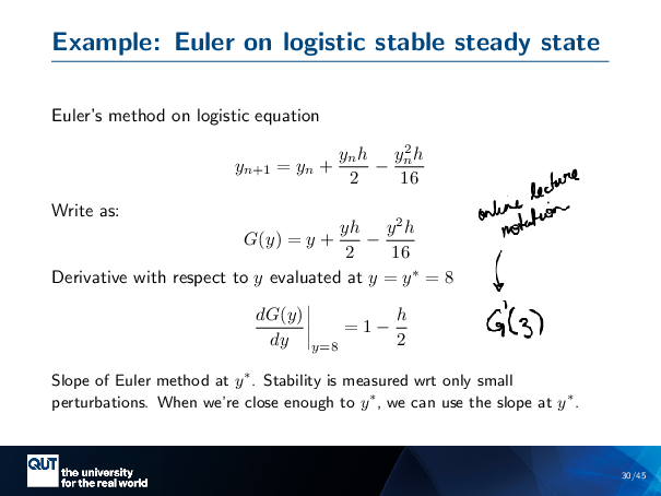
In your online lectures, you’ve got the Euler’s method on a Logistic Equation. So I’ve expanded it out here, just for convenience. And the first step is to write it as GY, so we’re replacing all these YNs with Ys. This is our G. And then you’re told that you take the derivative of G with respect to Y, evaluated at the steady state.
So in your online lectures, the notation used is this … So, hang on, what even is this? It’s okay, it’s the slope of G, it’s the slope of the Euler method at Y star.
So, if we were really, really close to our steady state, and we did a small perturbation, then we could kind of approximate what our map looks like as a line instead of the curve, and assume that the slope stays the same, provided we make our perturbation small enough. And so that’s the principle of stability analysis, it’s always with respect to a small enough perturbation that our maths is easy. And then we can use the slope of Y star.
So, let’s try applying this thing, and see if we can connect it back to the meaning.
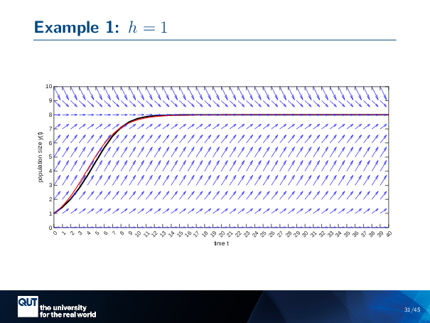
Figure scripts: plot_logistic_euler_red.m
This was our example before, where we had H equals 1, and it converged nicely and smoothly towards the steady state, the dynamical steady state. And so, if we …
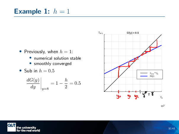
Figure scripts: plot_cobweb_stable.m
… take that, DGDY that we calculated before, and we substitute in H equals 0.5 … so we put an 0.5 in here … then we end up with 0.5 as our slope. And in fact that is giving us the same line as before that I did the cobweb plot on. I cheated, it’s the same example.
In this case, we know our Y star, it’s actually … equal to 8. And so what we do is we imagine ourselves perturbing our Euler’s method around this Y star just a little bit. So we start our perturbation here … And then we do … Just what we did before … visually.
And you see that even if we approach from above or below, our Euler’s method values get closer and closer to our Y star, until they’re kind of stuck there. And so this is our Euler’s method converging towards that dynamical steady state.
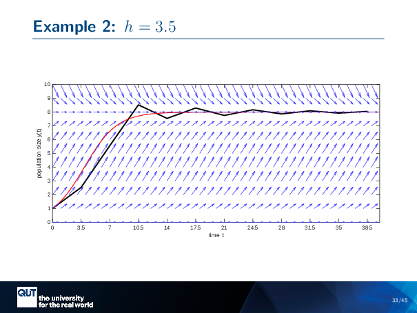
Figure scripts: plot_logistic_euler_red.m
Let’s take a look at the next example we had. This was when H equals 3.5, and it did converge, but it converged in this oscillatory way.
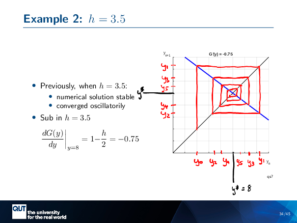
Figure scripts: plot_cobweb_osc_stable.m
So let’s use the derivative of G that we calculated before. We’re going to sub in here, this time, H equals 3.5 … so we put an 3.5 in here … and we get negative 0.75. So here’s our cobweb plot that we’re about to plot with the G slope at negative 0.75.
And so, if we do our iterations on this … so this here is, as before, Y star… Actually, I want to make that a little bit further down so that I’ll have space … And it’s the same on this side. So let’s say we start with our perturbation here at Y0, So we go … Up to here, this is our first Euler step, Y1. We’ll draw it on both axes. This is our next one, Y2 … Drew it on the other axis as well. That’s our Y3 … on axis as well. There’s our Y4 … Y5 … Y5 .. And so on.
Check it out. Looks like … Y0 was here… … Then for two, we jump to the other side. For three, we jump to the … of 1, I should say. For two, we jump to the other side, but a little bit closer. … 3, we jump to the other side, but a little bit closer …
It’s oscillating towards the steady-state. Which is exactly what we did when we looked at the quiver plots, right? It’s captured that dynamic for us.

Figure scripts: plot_logistic_euler_red.m
Let’s do one more example. So this was the one with H equals 4.5, and this one was unstable. It was oscillatory, and it diverged.
You think the cobweb plot looks cool? Yeah, same.
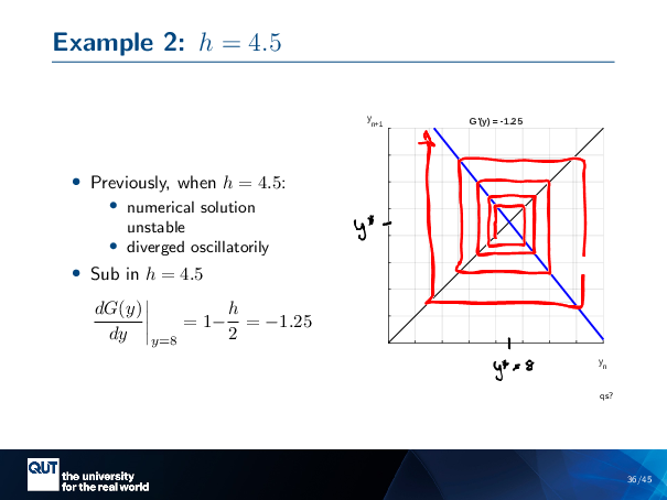
Figure scripts: plot_cobweb_unstable.m
So again, it’s the same thing. So we get … Our H equals 4.5, and we put it into our derivative here, and we’ve got negative 1.25, and so we’re drawing that line with a slope of negative 1.25.
This is our … Y star equals 8. Same thing here. This time, I’m going to start close. Because if I do the same process before … Horizontal 1, vertical blue, horizontal 1, Vertical G, horizontal 1, vertical G. You can see … there’s this same oscillatory thing happening, but the oscillations are getting bigger and bigger … And then it shoots off.
And so this cobweb plot and the pictures we’re drawing, is capturing what was happening in the Euler, in the numerical solutions dynamics.
At this point, are there any questions about what I’m doing there?
(A bit of back and forth with students)
… You all understand it really well. That’s good, because now you’re going to do your own.
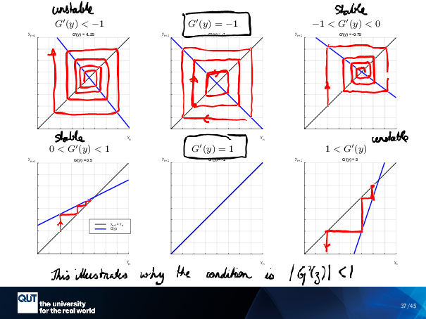
Figure scripts: plot_cobweb_unstable.m, plot_cobweb_neg1.m, plot_cobweb_osc_stable.m, plot_cobweb_stable.m, plot_cobweb_pos1.m, plot_cobweb_gt1.m
Okay, I’m going to send you to a pair-and-share. I’m going to send you guys to a breakout room.
I have already done … This one … and this one … and this one. I want you guys to do this one…. This one … And this one. This one’s the important one.
While you’re in the breakout room. Think about what the cobweb plot would look like, and what that means for the dynamics of the numerical solution near whatever steady state this is representing. And while you’re there, I’ll draw my own back in there as well, so that you’ll have something to look at how to do it. I’m gonna send you all away.
(Pair and share in class, breakout rooms online)
Okay, cool. Alright, so let’s go through them one by one. So what happens in this one here? If I … start off here, what did you guys notice about the … the cobweb plot that you end up with for this one. Comes back to where it started. Did you guys in chat find the same thing?
Okay, so we had a question about what happens in the cobweb plot with this one, and someone in the room said that it comes back to itself, and so that is indeed the case, that we end up going round. And, I have to make sure my lines are straight, and then we’re just going around in a circle, like this.
Alright, what about this one here, where G … the derivative of G equals 1? What happens with the dynamics in this one? … Yeah, like, not a lot, hey. So if you start here, there’s a line underneath… Are you just kind of stuck there? But they have the same intuition. Would it be a series of boxes inside each other for each initial value? Yeah, it’d just be a point, because it’s just stuck there for each initial value. This is like a weird edge case on the one. We’re going to return to this point of it being the one.
How about this one? The final one.
The top center graph? Oh, I’m sorry. Oh, yes, yes, you were right. Exactly true, that you would … if you started here, you would have another little limit cycle … going around like this. All the way around. Yeah, sorry, I thought you meant the one that I was talking about, the bottom center. That’s exactly right. Thanks.
And how about the final one? What does the dynamics look like for this one? Maybe if we start from here, what did you guys find? … Chat, you can beat them if you’re quick. … We figured it would go across to the right, then up, and repeat. Across to the right. No, see, yeah, so this is the only trick to the cobweb plot, is that you’ve got to remember that if you’re starting at the 1 to 1 line, then you’ve got to go vertical first. So you’re actually gonna go down like this. Because I was drawing the others on the left-hand side, wasn’t I? I mean, I drew it on the right-hand side here, but you’d basically have to do that same pattern here. So instead, you’d be going vertical down, and then across to the left. And then vertical down. And across to the left. And so, in this case, your Euler solution, so it always starts from that diagonal bisector. … Yeah, yeah, so the reason is because, remember when I was talking about it before? I said that this is my Y0…. Y0 here … And this was my Y1. And so I represented that by the vertical line from the one to the … to the G…. Yep.
Alright, cool, so we’ve kind of looked at the space of all of the possible slopes of G, And … We can say that this one is unstable … Numerical solution, the Euler method is unstable. This one is stable … it oscillates inwards. This one is stable … It converges inwards smoothly. And this one here is unstable.
So the thing that’s separating them, turns out, it’s these very edge cases here, when the derivative of G With respect to Y is negative 1, when the derivative of G with respect to Y is 1.
And so now, you remember that your online lectures, there was this rule about the G Z … Less … absolute value … less than 1. And now you know where that 1 is coming from! That’s why 1 separates them out. That’s the meaning of the stability of the fixed point and the Euler solution.
There’s a Menti quiz on the screen right now, and I’d be really grateful if you could just scan it into your phones or something and take the quiz. The reason is that this course is under development, and I get some input into it. And so basically, it’s just asking you, have you seen this stuff before? Yes or no, and was it useful to you anyway, or if it was new to you, was it useful to you in general?
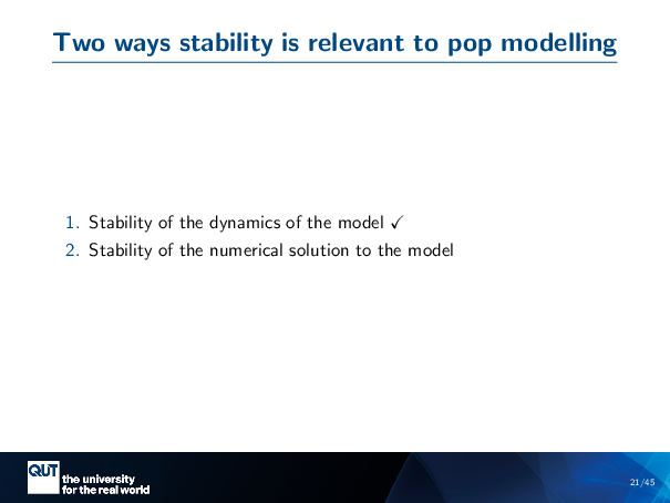
While we’re doing that, I’ll just talk about where we’ve been. We looked at the two ways that stability is relevant to population modelling.
The first way is the stability of the dynamics of the model itself. So, is a population at a steady state? Is that steady state for the population stable?
But then there’s also another layer that we put on top of it, which is our numerical method. We’re looking at Euler’s method only so far, but you will be looking at other methods in later online lectures. And all methods, eventually, are variations on Euler method, they build on this same principle, that you’re taking the derivative, you’re calculating the derivative and point, and you’re making some kind of jump.
You might be clever about it. You might take the average of derivatives over a space, or you might, go, oh, this derivative is too high, I’m going to take a smaller step at this point. But it’s all Euler methods at the bottom, all the way down.
And so we need to know about the stability of that numerical solution when it’s near the steady state, because, for instance, we might be interested in the step size. But then also later in the lectures, we leave this kind of iterative map to some really cool dynamics, like chaotic dynamics, period doubling chaos, which you’ll get a chance to look at in your practical.
That’s the end of that part, and now it’s time for activities…