Analytic solution for the stationary distribution in an iterated game with implementation errors
For the past year, I’ve been working in my spare time through a very interesting paper by Kleshnina et al. (2023). The paper concerns an evolutionary game theory model where individuals play an iterated Prisoner’s Dilemma with an environmental feedback. In a previous post, I experimented with a method to automate the identification of the subgame-perfect Nash equilibria and their parameter-value conditions.
In this post, I’ll show how the stationary distribution of actions taken during a repeated interaction can be found analytically and solved algorithmically using SymPy. The typical approach requires choosing a specific value for \(\varepsilon\), which is the probability that players make implementation errors. However, this choice is somewhat arbitrary if \(\varepsilon\) is introduced purely as a mathematical device to make the model tractable. My method avoids this arbitrariness by finding the limiting stationary distribution as \(\varepsilon \rightarrow 0\).
Kleshnina et al.’s paper concerns pairwise interactions that repeat over a number of rounds. The action that each player takes in each round is governed by their strategy, and it is a function of the actions in the previous round and the environmental state. If we assume that the probability \(\delta\) that the game continues for another round is high, then the payoff each strategy receives from interacting with each other strategy can be approximated. The approximation is made based on the stationary distribution of environment+action states when those two strategies interact.
To find the stationary distribution, Kleshnina et al. (2023) used a standard procedure, which is an approximate method. The Markov chain describing the sequence of environment+action states is not necessarily irreducible (e.g., Fig. 1). This means there are some states \(i\) that cannot reach another state \(j\) no matter how many rounds are played. Therefore, to find the stationary distribution, they assumed that in each round each player will make a mistake with probability \(\varepsilon\), playing cooperate instead of defect or vice versa. They set \(\varepsilon\) to a small fixed value, in their case \(\varepsilon = 0.01\), and modified the transition matrix accordingly. Then they found the left-eigenvector of the transition matrix numerically, which gives the stationary distribution.
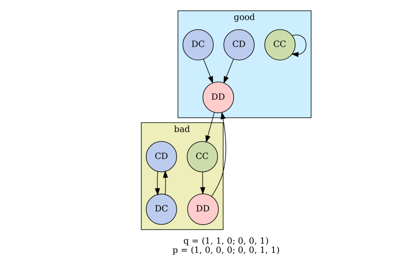
Figure 1. An example scenario that is not irreducible, where ‘good’ and ‘bad’ refer to the environment state, and the node labels refer to the players’ actions, ‘C’ for cooperate and ‘D’ for defect. The arrows indicate the transitions between environment+action states. For example, if the first round is in a good environment and Player 1 defects and Player 2 cooperates (DC), then the next round will also be in a good environment, and both players will defect. This scenario is reducible because some states cannot be reached from others. For example, the state good-CC can neither reach nor be reached from any other state.
Once all the stationary distributions between all pairs of strategies are found, the evolutionary dynamics can be solved. Each stationary distribution determines the payoff that both strategies receive when interacting with each other. These payoffs are then input to the evolutionary model, which describes how the population moves from fixation of one strategy to another over time. It is also a Markov chain model, and its stationary distribution gives the evolutionary steady state.
Fig. 2 below reproduces Fig. 3a from their paper, which shows the proportion of time selected strategies are at fixation at the evolutionary steady state. Some nodes in the figure are labelled with a binary string, which is a code that defines that strategy, while WSLS refers to the “win-stay lose-shift” strategy, and ALLD refers to “always defect”.
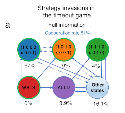
Figure 2. Adapted from Fig. 3a from Kleshnina et al. (2023), calculated for \(\varepsilon = 0.01\). The nodes are selected strategies, and the percentages are the proportion of time in the long-term that the population spends with that strategy at fixation.
The strategy proportions in Fig. 2 were calculated based on \(\varepsilon = 0.01\), and those proportions will change when \(\varepsilon\) changes (Fig. 3). In particular, as \(\varepsilon\) approaches zero, the proportion of time the population that pursues the most frequent strategy almost halves, and the relative ordering of the time proportions changes as well.
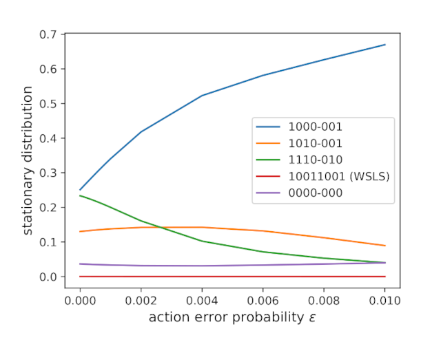
Figure 3. How the proportion of time spent at each strategy in Fig. 2 varies as a function of \(\varepsilon\). Note that the purple line that seems to correspond to ALLD in Fig. 2 is in fact strategy \(\boldsymbol{p} = (0, 0, 0, 0; -, 0, 0, 0)\), where the hyphen refers to a wildcard (can be 0 for defect or 1 for cooperate). ALLD, which has strategy \(\boldsymbol{p} = (0, 0, 0, 0; 0, 0, 0, 0)\), has half the proportion of the purple line shown. I couldn’t figure out the reason for the discrepancy.
Setting \(\varepsilon\) to some specific value may be valid depending on the question being asked. Nonetheless, in situations where \(\varepsilon\) is simply intended to represent “some small chance” of a mistake, then an intuitively attractive choice would be to find the solution as \(\varepsilon\) approaches zero. But that’s not something that’s easy to solve using numerical methods. It’s not obvious how close to \(\varepsilon = 0\) is “close enough”, and exploring the effects of different parameter values on the model is already computationally expensive. Furthermore, the smaller the value chosen for \(\varepsilon\) is, the more likely we are to run into numerical issues.
Instead, in the sections below, I detail how the stationary distribution as \(\varepsilon \rightarrow 0\) can be found analytically. In general, when the stationary distributions are found analytically, the evolutionary component of the model can predict quite different strategy proportions (Fig. 4). This also means that any conclusions we reach about which strategies are favoured by natural selection can depend on the method used.
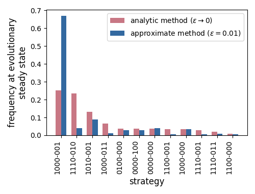
Figure 4. Comparing the evolutionary steady state when the analytic and approximate methods are used. Only the top 12 strategies are shown. Strategies are grouped into payoff-equivalent pairs, where a hyphen indicates that either cooperate or defect can be played.
The underlying principle to the analytic solution is illustrated in Example 1 below. Example 1 describes a somewhat different Markov chain scenario from the type they modelled, which I chose for its clarity. The section below works through a real example from their model, both by hand and in Python using SymPy.
Example 1. Consider a Markov chain with transition matrix
\[\begin{equation*} \boldsymbol{P} = \begin{pmatrix} 1 - \varepsilon & \varepsilon \\ \varepsilon & 1 - \varepsilon \\ \end{pmatrix}, \end{equation*}\]where \(\varepsilon\) is small. Show that, as \(\varepsilon \rightarrow 0\), the stationary distribution approaches
\[\boldsymbol{v}_{\varepsilon \rightarrow 0} \equiv \lim_{\varepsilon \rightarrow 0} \boldsymbol{v} = (1/2, 1/2).\] \[\star\]The stationary distribution \(\boldsymbol{v} = (v_1, v_2)\) satisfies
\[\begin{equation} \boldsymbol{v} = \boldsymbol{v} \; \boldsymbol{P}. \label{v=vP} \tag{1} \end{equation}\]We can write the elements of \(\boldsymbol{v}\) as polynomials of \(\varepsilon\)
\[\begin{align} v_1 &= k_{1, 0} + k_{1, 1} \varepsilon + k_{1, 2} \varepsilon^2 + \ldots \nonumber \\ v_2 &= k_{2, 0} + k_{2, 1} \varepsilon + k_{2, 2} \varepsilon^2 + \ldots \label{v0v1} \tag{2} \end{align}\]where \(k_{i,j}\) is the coefficient in the polynomial for state \(i\) of the \(j\)-th power of \(\varepsilon\). Then, as \(\varepsilon \rightarrow 0\), the stationary distribution will approach
\[\boldsymbol{v}_{\varepsilon \rightarrow 0} = (k_{1, 0}, k_{2, 0}).\]Our coefficients of interest represent probabilities, which gives us one equation describing the relationship between them
\[\begin{equation} 1 = k_{1, 0} + k_{2, 0}. \label{normalisation} \tag{3} \end{equation}\]To obtain more relationships, we can substitute Eq. \ref{v0v1} into Eq. \ref{v=vP} and equate matching-\(\varepsilon\)-order terms. We will increase the order until the coefficients defining \(\boldsymbol{v}_{\varepsilon \rightarrow 0}\) can be solved.
Substituting Eq. \ref{v0v1} into Eq. \ref{v=vP}
\[\begin{align*} v_1 &= \varepsilon (k_{2, 0} + k_{2, 1} \varepsilon + \ldots) + (1 - \varepsilon)(k_{1, 0} + k_{1, 1} \varepsilon + \ldots) \\ v_2 &= \varepsilon (k_{1, 0} + k_{1, 1} \varepsilon + \ldots) + (1 - \varepsilon)(k_{2, 0} + k_{2, 1} \varepsilon + \ldots) \end{align*}\]Substituting Eq. \ref{v0v1} on the left-hand side as well and expanding the right-hand side
\[\begin{align} k_{1, 0} + k_{1, 1} \varepsilon + k_{1, 2} \varepsilon^2 + \ldots &= k_{1,0} + \varepsilon(k_{2,0} -k_{1,0} + k_{1,1}) + \varepsilon^2 (k_{2,1} -k_{1,1} + \ldots) + \ldots \\ k_{2, 0} + k_{2, 1} \varepsilon + k_{2, 2} \varepsilon^2 + \ldots &= k_{2,0} + \varepsilon(k_{1,0} - k_{2,0} + k_{2,1}) + \varepsilon^2 (k_{1,1} - k_{2,1} + \ldots) + \ldots \label{expanded} \tag{4} \end{align}\]Matching the \(\varepsilon^0\) terms in Eq. \ref{expanded} gives us no useful information, so we increase the epsilon order. Matching the \(\varepsilon^1\) terms and simplifying, we obtain one new equation
\[\begin{equation} 0 = k_{1, 0} - k_{2, 0}. \label{eps1} \tag{5} \end{equation}\]We now have two linear equations to solve for two unknowns. Solving Eq. \ref{normalisation} and \ref{eps1} simultaneously, we obtain
\[\begin{align*} k_{1, 0} &= 1/2, \\ k_{2, 0} &= 1/2, \end{align*}\]and therefore
\[\begin{equation*} \boldsymbol{v}_{\varepsilon \rightarrow 0} = (1/2, 1/2). \end{equation*}\]Worked example
Consider a game played in the timeout environment
\[\boldsymbol{q} = ((1, 0, 0), (1, 1, 1))\]between two players, an All-Defect strategist
\[\boldsymbol{p}_0 = ((0, 0, 0, 0), (0, 0, 0, 0))\]and a peculiar, mostly-defecting strategy who only cooperates when the previous action was DD
\[\boldsymbol{p}_1 = ((0, 0, 0, 1), (0, 0, 0, 1)).\]Worked example by hand
Index the states: (1) gCC, (2) gCD, (3) gDC, (4) gDD, (5) bCC, (6) bCD, (7) bDC, (8) bDD.
In a deterministic game played without any errors, the transition matrix is
\[\begin{equation*} T = \begin{pmatrix} 0 & 0 & 0 & 1 & 0 & 0 & 0 & 0 \\ 0 & 0 & 0 & 0 & 0 & 0 & 0 & 1 \\ 0 & 0 & 0 & 0 & 0 & 0 & 0 & 1 \\ 0 & 0 & 0 & 0 & 0 & 0 & 1 & 0 \\ 0 & 0 & 0 & 1 & 0 & 0 & 0 & 0 \\ 0 & 0 & 0 & 1 & 0 & 0 & 0 & 0 \\ 0 & 0 & 0 & 1 & 0 & 0 & 0 & 0 \\ 0 & 0 & 1 & 0 & 0 & 0 & 0 & 0 \\ \end{pmatrix} \end{equation*}\]where rows are predecessors, columns are successors, and the state vector is multiplied on left.
The dynamics has two attractors — \(\{ \text{gDD}, \text{bDC} \}\) and \(\{ \text{bDD}, \text{gDC} \}\) — and the Markov chain is not irreducible (Fig. 5a).
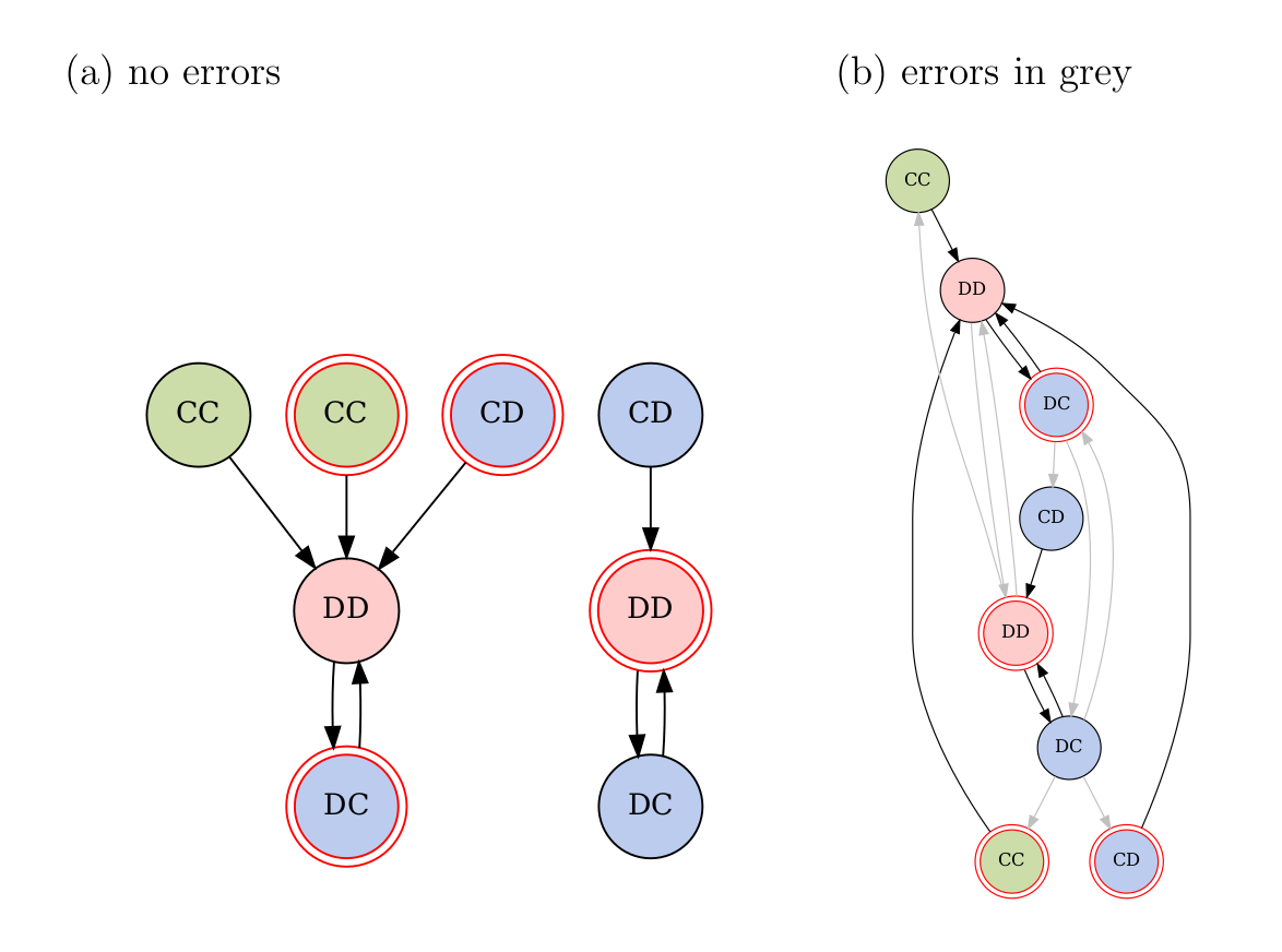
Figure 5. Environment+action state transition graphs for the current example. The environment is indicated by the border: a plain border is a good environment, and a double-ring red border bad. Actions are indicated by the text inside each node, with Player 1’s action first. (a) Transition graph when no action mistakes are made. This Markov chain is not irreducible. (b) Transition graph when errors are permitted, which are shown in grey. This chain is irreducible, and so the stationary distribution can be found. For clarity, only errors that are made in an attractor state are shown.
If players can make errors, then the Markov chain becomes irreducible (Fig. 5b). The transition matrix with the errors included is
\[\begin{equation*} P = \begin{pmatrix} \varepsilon^2 & \varepsilon(1 - \varepsilon) & \varepsilon(1 - \varepsilon) & (1 - \varepsilon)^2 & 0 & 0 & 0 & 0 \\ 0 & 0 & 0 & 0 & \varepsilon^2 & \varepsilon(1 - \varepsilon) & \varepsilon(1 - \varepsilon) & (1 - \varepsilon)^2 \\ 0 & 0 & 0 & 0 & \varepsilon^2 & \varepsilon(1 - \varepsilon) & \varepsilon(1 - \varepsilon) & (1 - \varepsilon)^2 \\ 0 & 0 & 0 & 0 & \varepsilon(1 - \varepsilon) & \varepsilon^2 & (1 - \varepsilon)^2 & \varepsilon(1 - \varepsilon) \\ \varepsilon^2 & \varepsilon(1 - \varepsilon) & \varepsilon(1 - \varepsilon) & (1 - \varepsilon)^2 & 0 & 0 & 0 & 0 \\ \varepsilon^2 & \varepsilon(1 - \varepsilon) & \varepsilon(1 - \varepsilon) & (1 - \varepsilon)^2 & 0 & 0 & 0 & 0 \\ \varepsilon^2 & \varepsilon(1 - \varepsilon) & \varepsilon(1 - \varepsilon) & (1 - \varepsilon)^2 & 0 & 0 & 0 & 0 \\ \varepsilon(1 - \varepsilon) & \varepsilon^2 & (1 - \varepsilon)^2 & \varepsilon(1 - \varepsilon) & 0 & 0 & 0 & 0 \\ \end{pmatrix} \end{equation*}\]For example, the \((1 - \varepsilon)^2\) in row \(i = 1\) (gCC) and column \(j = 4\) (gDD) means that the game will transition from gCC to gDD in the event that neither player makes an error, which occurs with probability \((1 - \varepsilon)^2\).
We can write the stationary distribution as a vector of polynomial functions of \(\varepsilon\)
\[\begin{equation} \boldsymbol{v}^T = \begin{pmatrix} v_1 \\ v_2 \\ \vdots \\ v_8 \\ \end{pmatrix} = \begin{pmatrix} k_{1, 0} + k_{1, 1} \varepsilon + k_{1, 2} \varepsilon^2 + k_{1, 3} \varepsilon^3 + \ldots \\ k_{2, 0} + k_{2, 1} \varepsilon + k_{2, 2} \varepsilon^2 + k_{2, 3} \varepsilon^3 + \ldots \\ \vdots \\ k_{8, 0} + k_{8, 1} \varepsilon + k_{8, 2} \varepsilon^2 + k_{8, 3} \varepsilon^3 + \ldots \\ \end{pmatrix} \label{Eq:stationary_distn_defn_v2} \tag{1} \end{equation}\]where \(k_{i,j}\) is the coefficient of the \(j\)-th power of \(\varepsilon\) in the polynomial describing the stationary distribution of state \(i\). As \(\varepsilon \rightarrow 0\), \(\boldsymbol{v} \rightarrow \boldsymbol{v}_{\varepsilon \rightarrow 0} = (k_{1,0}, k_{2,0}, \ldots, k_{8,0})\), so we are interested in finding the \(k_{i,0}\) coefficients.
The normalisation for the stationary distribution gives our first equation
\[\begin{equation} 1 = k_{1,0} + k_{2, 0} + \ldots + k_{8,0}. \label{Eq:normalised_k_0_to_7_v2} \tag{2} \end{equation}\]From Eq. \ref{Eq:stationary_distn_defn_v2}, we obtain 8 more equations
\[\begin{align*} k_{1, 0} + k_{1, 1} \varepsilon + \ldots & = \varepsilon^2 (\varepsilon k_{1,1} + k_{1,0}) + \varepsilon^2 (\varepsilon k_{5,1} + k_{5,0}) + \varepsilon^2 (\varepsilon k_{6,1} + k_{6,0}) + \varepsilon^2 (\varepsilon k_{7,1} + k_{7,0}) \\ & \quad + \varepsilon (1 - \varepsilon) (\varepsilon k_{8,1} + k_{8,0}) + \ldots \\ k_{2, 0} + k_{2, 1} \varepsilon + \ldots & = \varepsilon^2 (\varepsilon k_{8,1} + k_{8,0}) + \varepsilon (1 - \varepsilon) (\varepsilon k_{1,1} + k_{1,0}) + \varepsilon (1 - \varepsilon) (\varepsilon k_{5,1} + k_{5,0}) \\ & \quad + \varepsilon (1 - \varepsilon) (\varepsilon k_{6,1} + k_{6,0}) + \varepsilon (1 - \varepsilon) (\varepsilon k_{7,1} + k_{7,0}) + \ldots \\ & \vdots \\ k_{8, 0} + k_{8, 1} \varepsilon + \ldots & = \varepsilon (1 - \varepsilon) (\varepsilon k_{4,1} + k_{4,0}) + (1 - \varepsilon)^2 (\varepsilon k_{2,1} + k_{2,0}) + (1 - \varepsilon)^2 (\varepsilon k_{3,1} + k_{3,0}) + \ldots \end{align*}\]Grouping \(\varepsilon^0\) coefficients, we obtain 8 equations:
\[\begin{align*} k_{1,0} &= 0, \\ k_{2,0} &= 0, \\ k_{3,0} &= k_{8,0}, \\ k_{4,0} &= k_{1,0} + k_{5,0} + k_{6,0} + k_{7,0}, \\ k_{5,0} &= 0, \\ k_{6,0} &= 0, \\ k_{7,0} &= k_{4,0}, \\ k_{8,0} &= k_{2,0} + k_{3,0}, \end{align*}\]which, combined with the normalisation constraint (Eq.~\ref{Eq:normalised_k_0_to_7_v2}), can be reduced to the partial solution
\[\begin{align} \begin{split} k_{1,0} &= 0, \\ k_{2,0} &= 0, \\ k_{3,0} &= k_{8,0}, \\ k_{4,0} &= 1/2 - k_{8, 0}, \\ k_{5,0} &= 0, \\ k_{6,0} &= 0, \\ k_{7,0} &= 1/2 - k_{8, 0}. \end{split} \label{Eq:eps0_partial} \tag{3} \end{align}\]An unknown in \(\boldsymbol{v}_{\varepsilon \rightarrow 0}\) remains, so we consider the coefficients of the next power of \(\varepsilon\), which is \(\varepsilon^1\).
Grouping \(\varepsilon^1\) coefficients, we obtain 8 more equations
\[\begin{align} \begin{split} k_{1,1} &= k_{8,0}, \\ k_{2,1} &= k_{1,0} + k_{5,0} + k_{6,0} + k_{7,0}, \\ k_{3,1} &= k_{1,0} + k_{5,0} + k_{6,0} + k_{7,0} - 2 k_{8,0} + k_{8,1}, \\ k_{4,1} &= -2 k_{1,0} + k_{1,1} - 2 k_{5,0} + k_{5,1} - 2 k_{6,0} + k_{6,1} - 2 k_{7,0} + k_{7,1} + k_{8,0}, \\ k_{5,1} &= k_{4,0}, \\ k_{6,1} &= k_{2,0} + k_{3,0}, \\ k_{7,1} &= k_{2,0} + k_{3,0} - 2 k_{4,0} + k_{4,1}, \\ k_{8,1} &= -2 k_{2,0} + k_{2,1} - 2 k_{3,0} + k_{3,1} + k_{4,0} \end{split} \label{Eq:eps1} \tag{4} \end{align}\]Substituting Eqs. \ref{Eq:eps0_partial} into Eqs. \ref{Eq:eps1}, we obtain the remaining coefficients
\[\begin{align} \begin{split} k_{3,0} &= 3/14, \\ k_{4,0} &= 2/7, \\ k_{7,0} &= 2/7, \\ k_{8,0} &= 3/14. \end{split} \end{align}\]Therefore, as \(\varepsilon \rightarrow 0\), the stationary distribution approaches
\[\begin{equation} \boldsymbol{v}_{\varepsilon \rightarrow 0} = ( 0, 0, 3/14, 2/7, 0, 0, 2/7, 3/14). \end{equation}\]Worked example by code
Begin by defining the problem:
# A simplified script that calculates the solution for the worked example.
#
# The example has:
#   - q = (1, 0, 0; 1, 1, 1)
#   - p0 = (0, 0, 0, 0; 0, 0, 0, 0), ID = 0
#   - p1 = (0, 0, 0, 1; 0, 0, 0, 1), ID = 17

import sympy as sp
import numpy as np


# parameters
# ---

# epsilon is the action-error probability defined as a symbolic variable
eps = sp.symbols("eps")

# we will try to solve by matching coefficients of epsilon powers up to eps^2
max_pwr = 2

# the 8 x 8 transition matrix between states including errors
# (normally generated by other code, but hardcoded here for clarity)
P = np.array(
    [
        [eps**2, eps*(1 - eps), eps*(1 - eps), (1 - eps)**2, 0, 0, 0, 0],
        [0, 0, 0, 0, eps**2, eps*(1 - eps), eps*(1 - eps), (1 - eps)**2],
        [0, 0, 0, 0, eps**2, eps*(1 - eps), eps*(1 - eps), (1 - eps)**2],
        [0, 0, 0, 0, eps*(1 - eps), eps**2, (1 - eps)**2, eps*(1 - eps)],
        [eps**2, eps*(1 - eps), eps*(1 - eps), (1 - eps)**2, 0, 0, 0, 0],
        [eps**2, eps*(1 - eps), eps*(1 - eps), (1 - eps)**2, 0, 0, 0, 0],
        [eps**2, eps*(1 - eps), eps*(1 - eps), (1 - eps)**2, 0, 0, 0, 0],
        [eps*(1 - eps), eps**2, (1 - eps)**2, eps*(1 - eps), 0, 0, 0, 0]
    ],
    dtype=object
)
The first step to finding the stationary distribution is to define all our coefficients as symbolic variables
# find the stationary distribution
# ---

nbr_states = P.shape[0]

# matrix of epsilon coefficients, k_ij
#   - rows i correspond to the state
#   - columns j correspond to the power of epsilon
coeffs = [
    [sp.symbols(f"k{state_idx}{pwr}") for pwr in range(max_pwr + 1)]
    for state_idx in range(nbr_states)
]
This produces coeffs for \(\varepsilon\) up to the second power:
[[k00, k01, k02], [k10, k11, k12], [k20, k21, k22], [k30, k31, k32],
 [k40, k41, k42], [k50, k51, k52], [k60, k61, k62], [k70, k71, k72]]
Define the stationary distribution as a polynomial in epsilon up to max_pwr
# the stationary distribution expressed as a polynomial in epsilon
# v_i = k_i0 eps^0 + k_i1 eps^1 + ...
v = np.array(
    [
        sum(coeffs[state_idx][pwr] * eps**pwr for pwr in range(max_pwr + 1))
        for state_idx in range(nbr_states)
    ]
)
This produces v as a polynomial up to the second power:
array([eps**2*k02 + eps*k01 + k00, eps**2*k12 + eps*k11 + k10,
       eps**2*k22 + eps*k21 + k20, eps**2*k32 + eps*k31 + k30,
       eps**2*k42 + eps*k41 + k40, eps**2*k52 + eps*k51 + k50,
       eps**2*k62 + eps*k61 + k60, eps**2*k72 + eps*k71 + k70],
      dtype=object)
Define the right-hand side of the stationary distribution equation
# at the stationary distribution, v = vP
rhsV = list(v @ P)
This produces rhsV:
[eps**2*(eps**2*k02 + eps*k01 + k00) + eps**2*(eps**2*k42 + eps*k41 + k40) + eps**2*(eps**2*k52 + eps*k51 + k50) + eps**2*(eps**2*k62 + eps*k61 + k60) + eps*(1 - eps)*(eps**2*k72 + eps*k71 + k70),
 eps**2*(eps**2*k72 + eps*k71 + k70) + eps*(1 - eps)*(eps**2*k02 + eps*k01 + k00) + eps*(1 - eps)*(eps**2*k42 + eps*k41 + k40) + eps*(1 - eps)*(eps**2*k52 + eps*k51 + k50) + eps*(1 - eps)*(eps**2*k62 + eps*k61 + k60),
 eps*(1 - eps)*(eps**2*k02 + eps*k01 + k00) + eps*(1 - eps)*(eps**2*k42 + eps*k41 + k40) + eps*(1 - eps)*(eps**2*k52 + eps*k51 + k50) + eps*(1 - eps)*(eps**2*k62 + eps*k61 + k60) + (1 - eps)**2*(eps**2*k72 + eps*k71 + k70),
 eps*(1 - eps)*(eps**2*k72 + eps*k71 + k70) + (1 - eps)**2*(eps**2*k02 + eps*k01 + k00) + (1 - eps)**2*(eps**2*k42 + eps*k41 + k40) + (1 - eps)**2*(eps**2*k52 + eps*k51 + k50) + (1 - eps)**2*(eps**2*k62 + eps*k61 + k60),
 eps**2*(eps**2*k12 + eps*k11 + k10) + eps**2*(eps**2*k22 + eps*k21 + k20) + eps*(1 - eps)*(eps**2*k32 + eps*k31 + k30),
 eps**2*(eps**2*k32 + eps*k31 + k30) + eps*(1 - eps)*(eps**2*k12 + eps*k11 + k10) + eps*(1 - eps)*(eps**2*k22 + eps*k21 + k20),
 eps*(1 - eps)*(eps**2*k12 + eps*k11 + k10) + eps*(1 - eps)*(eps**2*k22 + eps*k21 + k20) + (1 - eps)**2*(eps**2*k32 + eps*k31 + k30),
 eps*(1 - eps)*(eps**2*k32 + eps*k31 + k30) + (1 - eps)**2*(eps**2*k12 + eps*k11 + k10) + (1 - eps)**2*(eps**2*k22 + eps*k21 + k20)]
Now we find equations that we can use to solve for the stationary distribution. The first equation is the normalisation equation
# At the stationary distribution, v = rhsV.
# As the error eps -> 0, the stationary distribution approaches
# the epsilon-order 0 coefficients, i.e.,
#   v -> (k_10, k_20, k_30, ...)

# solve by matching epsilon-power terms

# first, from normalisation of the stationary distribution,
# we always have: 1 = k_10 + k_20 + k_30 + ...
pwr_2_eq0s = {
    0: [1 - sum(coeffs[state_idx][0] for state_idx in range(nbr_states))]
}
So far, we have pwr_2_eq0s:
{0: [-k00 - k10 - k20 - k30 - k40 - k50 - k60 - k70 + 1]}
The other equations are obtained from \(\boldsymbol{v} = \boldsymbol{v}P\).
# then, from v = vP, each state has an equation involving various
# epsilon-order terms:
#   k_i0 + k_i1 eps + ... = [term]_i0 + [term]_i1 eps + ...
for state_idx, rhs in enumerate(rhsV):
    pwrs_terms = rhs.as_poly(eps).all_terms()
    for pwr_tuple, term in pwrs_terms:
        pwr = pwr_tuple[0]
        if pwr <= max_pwr:
            eq0 = term - coeffs[state_idx][pwr]
            if eq0 != 0:  # exclude not-useful 0 = 0 equations
                pwr_2_eq0s.setdefault(pwr, []).append(eq0)
Now, pwr_2_eq0s:
{0: [-k00 - k10 - k20 - k30 - k40 - k50 - k60 - k70 + 1,
  -k00,
  -k10,
  -k20 + k70,
  k00 - k30 + k40 + k50 + k60,
  -k40,
  -k50,
  k30 - k60,
  k10 + k20 - k70],
 1: [-k01 + k70,
  k00 - k11 + k40 + k50 + k60,
  k00 - k21 + k40 + k50 + k60 - 2*k70 + k71,
  -2*k00 + k01 - k31 - 2*k40 + k41 - 2*k50 + k51 - 2*k60 + k61 + k70,
  k30 - k41,
  k10 + k20 - k51,
  k10 + k20 - 2*k30 + k31 - k61,
  -2*k10 + k11 - 2*k20 + k21 + k30 - k71],
 2: [k00 - k02 + k40 + k50 + k60 - k70 + k71,
  -k00 + k01 - k12 - k40 + k41 - k50 + k51 - k60 + k61 + k70,
  -k00 + k01 - k22 - k40 + k41 - k50 + k51 - k60 + k61 + k70 - 2*k71 + k72,
  k00 - 2*k01 + k02 - k32 + k40 - 2*k41 + k42 + k50 - 2*k51 + k52 + k60 - 2*k61 + k62 - k70 + k71,
  k10 + k20 - k30 + k31 - k42,
  -k10 + k11 - k20 + k21 + k30 - k52,
  -k10 + k11 - k20 + k21 + k30 - 2*k31 + k32 - k62,
  k10 - 2*k11 + k12 + k20 - 2*k21 + k22 - k30 + k31 - k72],
}
We write the list of coefficients we want to solve for
# we only want to solve the values of k_10, k_20, ...
wants = [coeffs[state_idx][0] for state_idx in range(nbr_states)]
This produces wants:
[k00, k10, k20, k30, k40, k50, k60, k70]
We incrementally increase the maximum epsilon power until we have an expression for each of the coefficients we want with no free symbols
# so we match epsilon terms, increasing the epsilon power
# incrementally, until we have taken into account enough rare
# sequences of errors that we can obtain the solutions we want
stationary_distn = list()
eq0s = list()
for pwr_level in range(max_pwr+1):

    # add to our system of equations
    # coefficient-matching at current power level
    eq0s += pwr_2_eq0s[pwr_level]

    # solve system of equations for epsilon coefficients
    free_coeffs = set.union(*[eq0.free_symbols for eq0 in eq0s])
    soln = sp.solve(eq0s, free_coeffs) # returns [] if can't

    # check if solution has all the coefficients we want
    if all(want in soln for want in wants):
        # got an expression for each coeff we wanted
        stationary_distn_temp = [soln[want] for want in wants]
        if all([not propn.free_symbols for propn in stationary_distn_temp]):
            # each an expression we got had no unknown variables, so we're done!
            stationary_distn = stationary_distn_temp
            break
The loop above breaks at pwr_level = 1,
giving soln:
{k00: 0, k01: 3/14, k10: 0, k11: 2/7, k20: 3/14, k21: k71 - 1/7, k30: 2/7,
 k31: k61 + 5/14, k40: 0, k41: 2/7, k50: 0, k51: 3/14, k60: 2/7, k70: 3/14}
And so the stationary distribution as \(\varepsilon \rightarrow 0\) is stationary_distn:
[0, 0, 3/14, 2/7, 0, 0, 2/7, 3/14]
Future work
One thing I’m unclear about is how to determine the maximum power max_pwr that is needed to find the solution.
My intuition tells me that the maximum power is probably the maximum number of errors needed to escape from one attractor to another, such that all attractors are eventually reachable.
One could check only the states in each attractor
for their shortest route to other basins.
However, the shortest route of escape might pass through a transient state in the attractor’s own basin.
Though even if that’s the case, it might not matter for much practical purposes;
there’s no great harm in overestimating max_pwr, as I do in the example code above,
it just means more computations.
I’m sure that someone has used this method before, but I haven’t been able to find it in the literature. I found a book Kato (1980), which has Chapter 2 dedicated to perturbation theory; however, the form of perturbation it considers is different from the one I use here. I also found Kandori et al. (1993), which has a very similar-looking polynomial; however, their method seems to require finding all possible structures they call “z-trees”, which is computationally expensive.
References
Kandori, M., Mailath, G. J. and Rob, R. (1993). Learning, mutation, and long run equilibria in games. Econometrica: Journal of the Econometric Society, 61(1):29-56.
Kato, T. (1980) Perturbation Theory for Linear Operators. Springer-Verlag, Berlin.
Kleshnina, M., Hilbe, C., Šimsa, Š., Chatterjee, K. and Nowak, M.A. (2023). The effect of environmental information on evolution of cooperation in stochastic games. Nature Communications, 14(1):4153.