Check if an iterated Prisoner's Dilemma strategy is a subgame perfect Nash equilibrium

I recently read a paper by Kleshnina et al. (2023), The effect of environmental information on evolution of cooperation in stochastic games, which provided an opportunity to teach myself about how to analyse iterated games. In particular, the problem they investigated admits 64 possible scenarios with 256 possible strategies each, and I was interested in writing code that could automate the analysis. The solution I eventually landed on (Github repo) used a combination of SymPy, NetworkX, SageMath, the Z3 Theorem Prover, and PyEDA for Boolean minimisation, but I think my approach could be improved.

Background to the paper

Kleshnina et al. (2023) studied an iterated Prisoner’s Dilemma (PD) where the actions of the players affect the environment and visa versa. Typically, if the environment is good, the players receive higher payoffs, but if some players defect, then the environment transitions from good to bad. They were interested in what effect knowledge of the environment’s state would have on cooperation outcomes. Here, however, I will focus on one small aspect of the methodology: how to identify if a strategy is a sub-game perfect Nash equilibrium and the conditions required. This is the focus of Supplementary Note 3.

Game structure

Two players are playing an iterated a Prisoner’s Dilemma (PD), where in each round they can either cooperate (C) or defect (D). The environment has two possible states, \(S = \{ s_1, s_2 \}\), or ‘good’ and ‘bad’, respectively. The environment state determines payoffs according to the tables below, where \(b_1 > b_2 > c\).

In the good environment:

	C	D
C	\(b_1 - c\)	\(-c\)
D	\(b_1\)	\(0\)

In the bad environment:

	C	D
C	\(b_2 - c\)	\(-c\)
D	\(b_2\)	\(0\)

Environment transitions

I will focus on the scenario where the environment is deterministic and changes state depending on its previous state and the players’ actions. In each round, the environment will either transition to the good state or the bad state. To represent this mathematically, let \(q_{a, \overline{a}}^i\) be an indicator variable given the previous environment state \(i\) and player actions \(a, \overline{a}\). When \(q_{a, \overline{a}}^i = 1\), the environment will transition to the good state in the next round; when \(q_{a, \overline{a}}^i = 0\), it will transition to the bad state. The complete set of possible transitions can be represented by the vector:

\[\boldsymbol{q} = ( q_{CC}^1, q_{CD}^1, q_{DD}^1; q_{CC}^2, q_{CD}^2, q_{DD}^2 ).\]

I will also focus on the full-information setting, where players actions depend on both the current environment state as well as the players’ previous actions (memory-1). Similar to the environment transitions, we use an indicator variable \(p_{a, \overline{a}}^j\) to represent a player’s decision in state \(j\) given previous actions \(a, \overline{a}\). Here, \(p_{a, \overline{a}}^j = 1\) indicates cooperation and \(p_{a, \overline{a}}^j = 0\) indicates defection. A player’s complete strategy can therefore be represented by the vector:

\[\boldsymbol{p}_F = ( p_{CC}^1, p_{CD}^1, p_{DC}^1, p_{DD}^1; p_{CC}^2, p_{CD}^2, p_{DC}^2, p_{DD}^2 ).\]

Player strategies

In Supplementary Note 3, Kleshnina et al. study what they call the ‘timeout’ game. In this game, if any player defects, both are penalised by spending one round in the bad environment. This mechanism can be represented by the transition vector:

\[\boldsymbol{q} = (1, 0, 0; 1, 1, 1).\]

They analyse several strategies in this setting, including one that combines two well-known approaches: playing ‘Grim’ in the good environment and ‘win-stay, lose-shift (WSLS)’ in the bad environment. This hybrid strategy is represented by the vector:

\[\boldsymbol{p} = (1, 0, 0, 0; 1, 0, 0, 1)\]

One-shot deviation analysis

Kleshnina used the one-shot deviation principle to determine when the Grim-WSLS strategy in the timeout environment is a sub-game perfect Nash equilibrium (SPNE). Her analysis examines every possible combination of previous actions and current environment state (e.g., (CC, good), (CD, good), (DC, good), …, (DC, bad), (DD, bad)). For each combination, we calculate:

• \(\pi_{a \overline{a}, i}\): the payoff for following the strategy
• \(\hat{\pi}_{a \overline{a}, i}\): the payoff for deviating from the strategy for one round
• \(\pi_{a \overline{a}, i} - \hat{\pi}_{a \overline{a}, i}\): the net benefit of staying with the strategy

For the strategy to qualify as a SPNE, it must always be more profitable to stick with the strategy than to deviate from it for even a single round. Mathematically, this means:

\[\pi_{a \overline{a}, i} - \hat{\pi}_{a \overline{a}, i} \geq 0 \text{ for all } (a \overline{a}, i).\]

As an example, consider the payoffs of the non-deviating and deviating players starting at CC in the good environment. For the non-deviating case, if both players start at CC, then they will cooperate in all subsequent rounds. The payoff will be

\[(b_1-c) + \delta(b_1-c) + \delta^2 (b_1-c) + \ldots,\]

where \(\delta\) is the probability of playing another round. Game theorists often use a \((1- \delta)\) normalisation to simplify the analysis. So the non-deviating payoff is calculated:

\[\begin{align*} \pi_{\text{CC, good}} &= (1 - \delta) \left( (b_1-c) + \delta(b_1-c) + \delta^2 (b_1-c) + \ldots \right),\\ &= (b_1 - c) \underbrace{(1 - \delta) \left( 1 + \delta + \delta^2 + \ldots \right)}_{=1}, \\ \pi_{\text{CC, good}} &= b_1 - c. \end{align*}\]

To calculate the one-shot deviation payoff, we calculate what the payoff would be if the focal player plays the opposite of what their strategy says for just one round, i.e., instead of C they play D, and the next round and then revert to their strategy.

The payoff in each round is tabulated below

	0	1	2	3	4	5	…
state	1	1	2	1	2	1	…
player 1	C	D	D	D	C	C	…
player 2	C	C	D	D	C	C	…
state transn	100; 111	100; 111	100; 111	100; 111	100; 111	100; 111	…
strat. transn	1000; 1001	1000; 1001	1000; 1001	1000; 1001	1000; 1001	1000; 1001	…
payoff		\(b_1\)	0	0	\(b_2 - c\)	\(b_1 - c\)	…

The actual payoff is

\[b_1 + \delta^3(b_2-c) + \delta^4( b_1 - c + \delta^1 (b_1 - c) + \ldots),\]

which normalises to

\[\hat{\pi}_{\text{CC, good}} = b_1(1-\delta) + \delta^3(b_2-c)(1-\delta) + \delta^4( b_1 - c ).\]

Therefore, from the (CC, good) starting point, we obtain a condition for the strategy to be a SPNE

\[\pi_{\text{CC, good}} - \hat{\pi}_{\text{CC, good}} = b_1 \delta (1 - \delta^3) - b_2 \delta^3 (1 - \delta) - c(1 - \delta^3) \geq 0. \label{1} \tag{1}\]

To simplify the condition, Kleshnina et al. take the limit as \(\delta \rightarrow 1\), which represents a kind of best-case scenario to identify a necessary condition. First we pull out common \(1-\delta\) terms

\[\pi_{\text{CC, good}} - \hat{\pi}_{\text{CC, good}} = (1 - \delta) \{ b_1 \delta (1 + \delta + \delta^2) - b_2 \delta^3 - c (1 + \delta + \delta^2) \},\]

and as \(\delta \rightarrow 1\), the condition becomes

\[\lim_{\delta \rightarrow 1} (\pi_{\text{CC, good}} - \hat{\pi}_{\text{CC, good}}) = 3 b_1 - b_2 - 3 c \geq 0. \label{2} \tag{2}\]

The analysis above is repeated for every possible combination (CC, good), (CD, good), …, (DD, bad). Kleshnina et al. find that the condition is satisfied for all other combinations except (DD, bad), which, in a similar way to (CC, good) above, results in a condition

\[\lim_{\delta \rightarrow 1} (\pi_{\text{DD, good}} - \hat{\pi}_{\text{DD, good}}) = 2 b_1 - b_2 - 2 c \geq 0. \label{3} \tag{3}\]

Both of the conditions must be satisfied in order for the strategy to be a SPNE. However, we can simplify the analysis by determining relationship between the two conditions. Eq. 2 can be rewritten \(b_1 - c + 2 b_1 - b_2 - 2 c \geq 0\). Because \(b_1 > c\), we know that if Eq. 3 is satisfied, then Eq. 2 is satisfied. Therefore, Eq. 3 is the necessary condition for the strategy to be a SPNE.

Automating the analysis

In the kleshnina-2023-playground Github repository, I provide code that automates analysis above for an arbitrary environment \(\boldsymbol{q}\) and strategy \(\boldsymbol{p}\). Below, I will highlight some points of interests, and I also note areas that I’m uncertain about / could be improved.

Encoding the environment and strategy as a directed graph

I used NetworkX to encode every \((\boldsymbol{q}, \boldsymbol{p})\) as a directed graph. The nodes are the environment-state + action pairs, e.g., (CC, good), and the edges are the transitions between them. Fig. 1 below shows the Timeout-Grim-WSLS example from above.

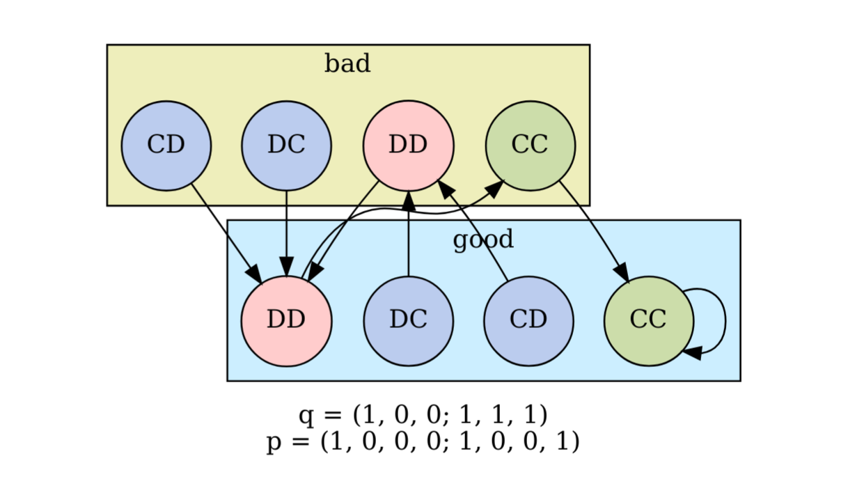
Figure 1. State transitions for the Grim-WSLS strategy played in the Timeout environment. Generated using dottify_state_space() in fncs_general.py.

Identifying attractors

In the Timeout-Grim-WSLS example above, the state (CC, good) is a steady state – once reached, players continue to cooperate and the environment remains good. However, it’s also possible to have periodic states that cycle through multiple configurations.

Consider an environment

\[\boldsymbol{q} = (1, 1, 0; 0, 0, 1),\]

and the strategy

\[\boldsymbol{p} = (1, 0, 0, 0; 0, 0, 1, 1).\]

As illustrated in Fig. 2 below, this system has three attractors:

1. A steady state or period-1 cycle: (CC, good) \(\rightarrow\) (CC, good) \(\rightarrow\) …
2. A period-2 cycle: (CD, bad) \(\rightarrow\) (DC, bad) \(\rightarrow\) (CD, bad) \(\rightarrow\) …
3. A period-3 cycle: (CC, bad) \(\rightarrow\) (DD, bad) \(\rightarrow\) (DD, good) \(\rightarrow\) (CC, bad) \(\rightarrow\) …

We need to identify such cyles, and we will find that the normalisation used above no longer applies.

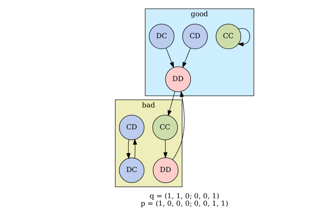
Figure 2. An example scenario with attractors that are period-1, period-2, and period-3 cycles.

To identify cycles, I used the strongly_connected_components() function from NetworkX. A strongly connected component (SCC) is a subgraph of a directed graph that has a path in each direction between each pair of vertices and is maximal with respect to this property. This function returns multi-node cycles plus SCCs of length 1. SCCs of length 1 may either be a node with no incoming links or a period-1 cycle. This is implemented in the find_cycles() function in fncs_general.py.

def find_cycles(G):

    # find the attractors using the strongly-connected components algorithm
    sccs = list(nx.strongly_connected_components(G))
    cycles = []
    for scc in sccs:
        if len(scc) > 1:
            # multi-node SCCs are always cycles
            cycles.append(scc)
        elif len(scc) == 1:
            node = list(scc)[0]
            # an SCC of size 1 is a steady-state iff it's a self-loop
            if G.has_edge(node, node):
                cycles.append({node})

    return cycles

Returning to our example in Fig. 2, we find that the normalisation factor \((1 - \delta)\) no longer applies. For example, the unnormalised no-deviation payoff from (CD, good) is

\[\begin{align*} \pi_{\text{CD, good}} &= \delta 0 + \delta^2(b_2 - c) + \delta^3 0 + \delta^4 0 + \ldots, \\ &= \delta \left( \frac{\delta (b_2 - c)}{1- \delta^3} \right). \\ \end{align*}\]

Therefore, when the payoffs are calculated in calc_longterm_payoffs() (in fncs_general.py), we leave them in their unnormalised form and perform the simplifications later when the conditions are evaluated (in SageMath, detailed below).

Calculating the no-deviation and deviation payoffs

I encoded the payoffs using SymPy (calc_one_shot_devns.py), and checked the conditions using SageMath (define_variables_assumptions.sage and check_spne.sage). To replicate the analysis done in Supplementary Note 3, I did the checking of the conditions incrementally, proceeding to the next step if the previous result was ambiguous.

1. Check the SPNE condition directly: Can SageMath immediately discern the sign of \(\pi_{a \overline{a}, i} - \hat{\pi}_{a \overline{a}, i}\)?
2. Use SageMath function numerator_denominator() to cancel the normalisation factors. Can SageMath discern the sign of each?
   • Note that I’m uncertain about the robustness of this step because it performs the simplifications I need as kind of side-effect of creating the fractional form and splitting it.
3. Simplify by setting \(\delta = 1\). Can SageMath discern the sign of \(\lim_{\delta \rightarrow 1} \pi_{a \overline{a}, i} - \hat{\pi}_{a \overline{a}, i}\)?
4. Write the condition from Step 3 to a file.

I found that SageMath had difficulty working in the \((b_1, b_2, c)\) parameter space, so I shifted to an \((x, y, c)\) parameter space defined as

\[\begin{align*} x &= b_2 - c, \\ y &= b_1 - b_2, \end{align*}\]

with the constraints \(x, y > 0\).

I don’t feel very confident about the SageMath implementation. I made an attempt to rewrite it in Z3, but I ran into difficulties because Z3 does not have an equivalent to SageMath’s numerator_denominator() function. Perhaps I can use some combination of SymPy and Z3 for this step. This is an area for future improvement.

For each \(\boldsymbol{q}\), output was a CSV file (one_shot_devns_q_[binary string].csv):

p	not_SPNE	gCC_satisfied?	gCC_how_determined?	gCC_required_non_negative	…
_00000000	False	True	directly	c	…
_00000001	True	True	directly	(b2 - c)d^2/(d^2 - 1) + c - (b2 - c)d/(d^2 - 1)	…
…	…	…	…	…	…

Calculate the necessary conditions

For each strategy that had the potential to be a SPNE in environment \(\boldsymbol{q}\), I used the Z3 Theorem Prover to determine which of the conditions (arising from each (CC,good), (CD, good), etc.) were the necessary conditions. In other words, I am analysing the relationships between the expressions arising from the requirement \(\pi_{a \overline{a}, i} - \hat{\pi}_{a \overline{a}, i} \geq 0\), such as the condition \(3 b_1 - b_2 - 3 c \geq 0\) in the Timeout-Grim-WSLS example.

For each strategy, the initial steps were:

First, identify all unique conditions using are_equivalent() in fncs_z3_1.py:

def are_equivalent(condn_a, condn_b):
    """
    Returns True if condn_a and condn_b and equivalent.
    """

    s = Solver()
    s.add(condn_a != condn_b)
    result = s.check() == unsat

    return result

Second, check if the unique conditions are mutually satisfiable (in calc_necess_condns.py):

# earlier in the code, specify assumptions on parameters
b1, b2, c, d = Reals("b1 b2 c d")
variables = [b1, b2, c, d]
assumptions = And(
    d > 0,
    d <= 1,
    c > 0,  # b1 ≥ b2 > c
    b2 > c,
    b1 > b2, # NOTE I changed this from Maria's b1 >= b2
)

# for each strategies unique conditions ...

# check conditions' mutual satisfiability
s = Solver()
s.add(assumptions)
for condn in condns:
    s.add(condn)
result = s.check()

If the conditions were mutually satisfiable, I then identified the minimal set of conditions that were the necessary conditions for that strategy. For each pair of conditions \(C_1\) and \(C_2\), I used Z3’s qe Tactic to determine if \(C_1 \implies C_2\), implemented in check_implication():

# in the script that calls the function, specify we're using 'qe' tactic
tactic = Tactic("qe")

# for each pair of conditions, call this function
def check_implication(condn_a, condn_b, assumptions, variables, tactic):
    """
    Returns True if condn_a implies condn_b under the given assumptions
    """

    formula = ForAll(variables, Implies(And(assumptions, condn_a), condn_b))
    result = tactic.apply(formula)

    return result.as_expr()

This allowed me to construction an implications matrix, which has rows and columns corresponding to the conditions, and an entry 1 indicates that \(C_i \implies C_j\). The minimal set is the set of all conditions that are not implied by another condition, i.e., the independent roots of the implications tree.

The results were stored in CSV files necess_condns_q_[binary string].csv. The Timeout environment example (necess_condns_q_100111.csv) is shown below.

p	simul_sat?	necessary_conditions	necessary_conditions_xy
_00000000	True
_00001000	True
_10000000	True
_10000001	True	2b1 - b2 - 2c	-1c + x + 2y
_10000111	True	b1 - b2 - c	y + -1*c
_10001000	True
_10001001	True	2b1 - b2 - 2c	-1c + x + 2y
_10001111	True	b1 - b2 - c	y + -1*c
_10010000	True	b1 - 2*c	-1*c + x + y
_10010001	True	b1 - 2*c	-1*c + x + y
_10010110	True	b1 - b2 - c | -b2 + 2*c	y + -1c | c + -1x
_10010111	True	b1 - b2 - c	y + -1*c
_10011000	True	b1 - 2*c	-1*c + x + y
_10011001	True	b1 - 2*c	-1*c + x + y
_10011110	True	b1 - b2 - c | -b2 + 2*c	y + -1c | c + -1x
_10011111	True	b1 - b2 - c	y + -1*c
_11110000	True	b1 - 2*c	-1*c + x + y
_11111000	True	b1 - 2*c	-1*c + x + y

Grouping same-condition strategies

Often, different strategies \(\boldsymbol{p}\) have the same necessary conditions. To further summarise the analysis, I grouped all such \(\boldsymbol{p}\) together using PyEDA’s Boolean minimisation on the set of \(\boldsymbol{p}\) binary strings.

For example, in the Timeout environment, the \(\boldsymbol{p}\) corresponding to the following 4 binary strings have no additional conditions in order to be a SPNE:

00000000
00001000
10000000
10001000

These four strings can be represented in a more compact form by a single string

-000-000

where the - indicates that the strategy can either cooperate or defect in that state.

The Boolean minimisation was implemented in group_necess_condns.py and output was written to CSV files necess_condns_grouped_q_[binary string].csv. The Timeout environment example (necess_condns_grouped_q_100111.csv) is shown below.

id	necessary_conditions	necessary_conditions_xy	compact_ps
0			_-000-000
1	2b1 - b2 - 2c	-1c + x + 2y	_1000-001
2	b1 - b2 - c	y + -1*c	_100–111
3	b1 - 2*c	-1*c + x + y	_1111-000 | _1001-00-
4	b1 - b2 - c | -b2 + 2*c	y + -1c | c + -1x	_1001-110

I wrote scripts plot_necess_condns.py and plot_transn_graphs_pq.py to visualise each \(\boldsymbol{p}\) group and its necessary conditions. I found it more convenient to work in the \((x, y)\) parameter space for the conditions.

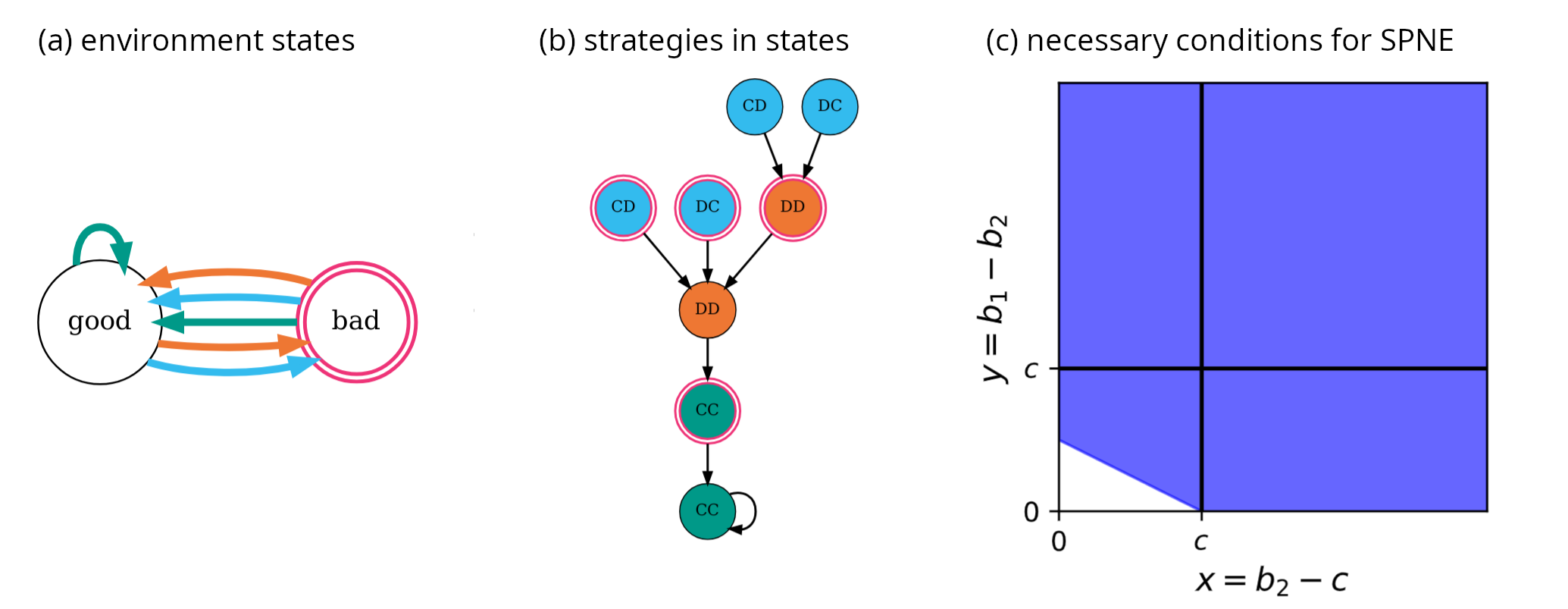
Figure 3. Summary analysis of Grim-WSLS and Grim-Risker strategy played in the Timeout environment. Panels show (a) the Timeout environment state transitions, (b) the state transitions that result from the combined Grim-WSLS and Grim-Risker strategies played in the Timeout environment, and (c) the region of parameter space (purple) that satisfies the necessary condition for the strategies to be a SPNE.

A summary of all SPNE in sensible environments

With code to automate the analysis, it is possible to do a sweep of a range of scenarios quickly. Below, I show the results I obtained for all environments with a ‘sensible’ transition pattern, i.e., that stay in or return to the good environment when both players cooperate and stay or return to the good environment when both players defect. These environments match the pattern

\[\boldsymbol{q} = (1, -, 0; 1, -, 0).\]

Figs. 4–6 below summarise the SPNE I found in each environmental scenario.

Environments are categorised based on how fragile they are and their return conditions. A fragile environment transitions from good to bad when any player defects, but a resilient environment only transitions when both players defect.

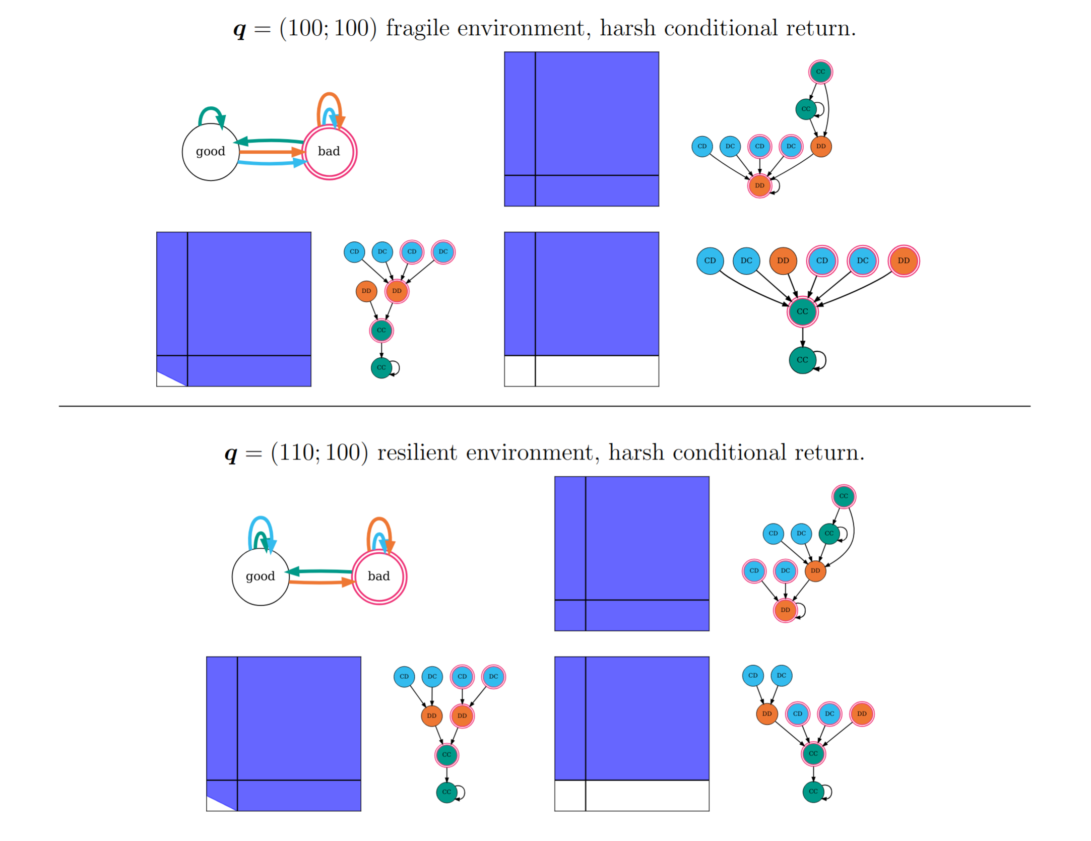
Figure 4. SPNE in harsh conditional return environments. From left to right, top to bottom, the \(\boldsymbol{p}\)-groups in the fragile environment are -----000, 1----001, and 1----111; and in the resilient environment are -00--000, 100--001, and 100--111

The conditions for return from the bad to good environment can be classified as:

1. harsh conditional – both players must cooperate,
2. conditional – at least one player must cooperate, or
3. timeout – returns regardless of what players do.

In all environments, a variation that always defects in the bad environment in response to any defection in the previous round is an unconditional SPNE.

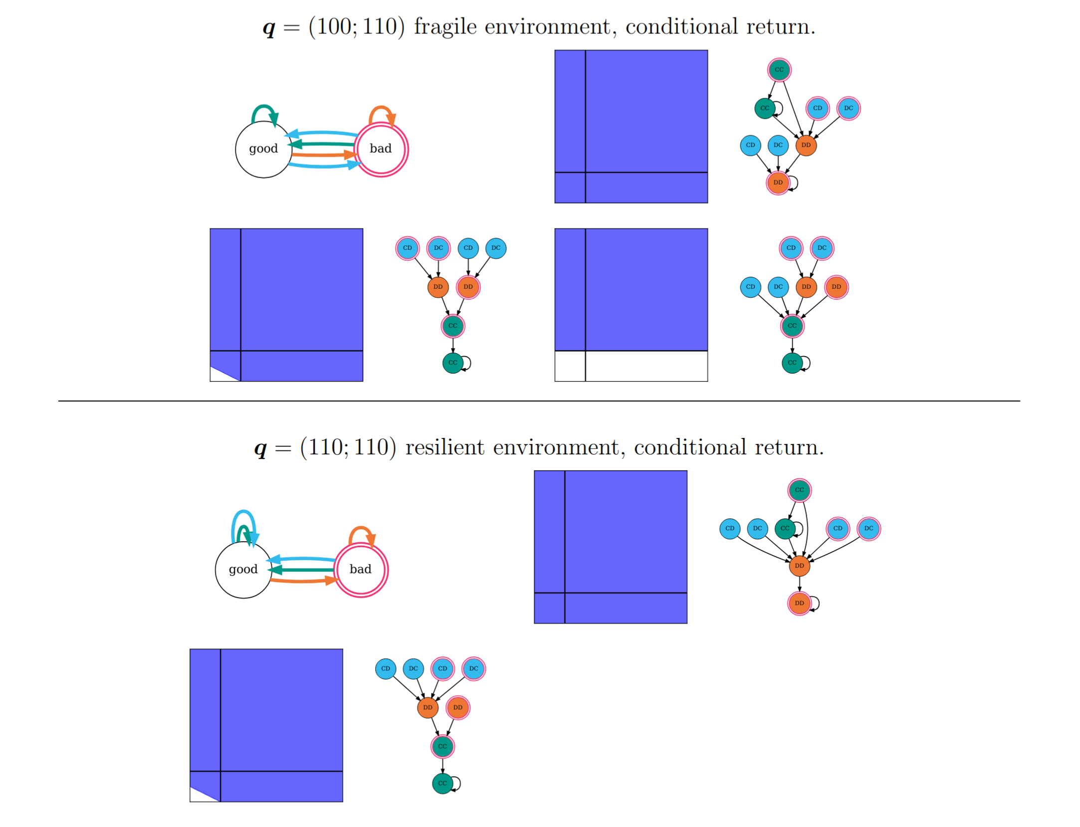
Figure 5. SPNE in conditional return environments. From left to right, top to bottom, the \(\boldsymbol{p}\)-groups in the fragile environment are -00--000, 100--001, and 100--111; and in the resilient environment are -00----0 and 100----1

All other potential SPNE are conditional and have (CC, good) as an attractor. In the resilient environment, they have in common a 100... pattern, which means that, if they are in the good environment, they respond to defection by the other in the previous round with a defection.

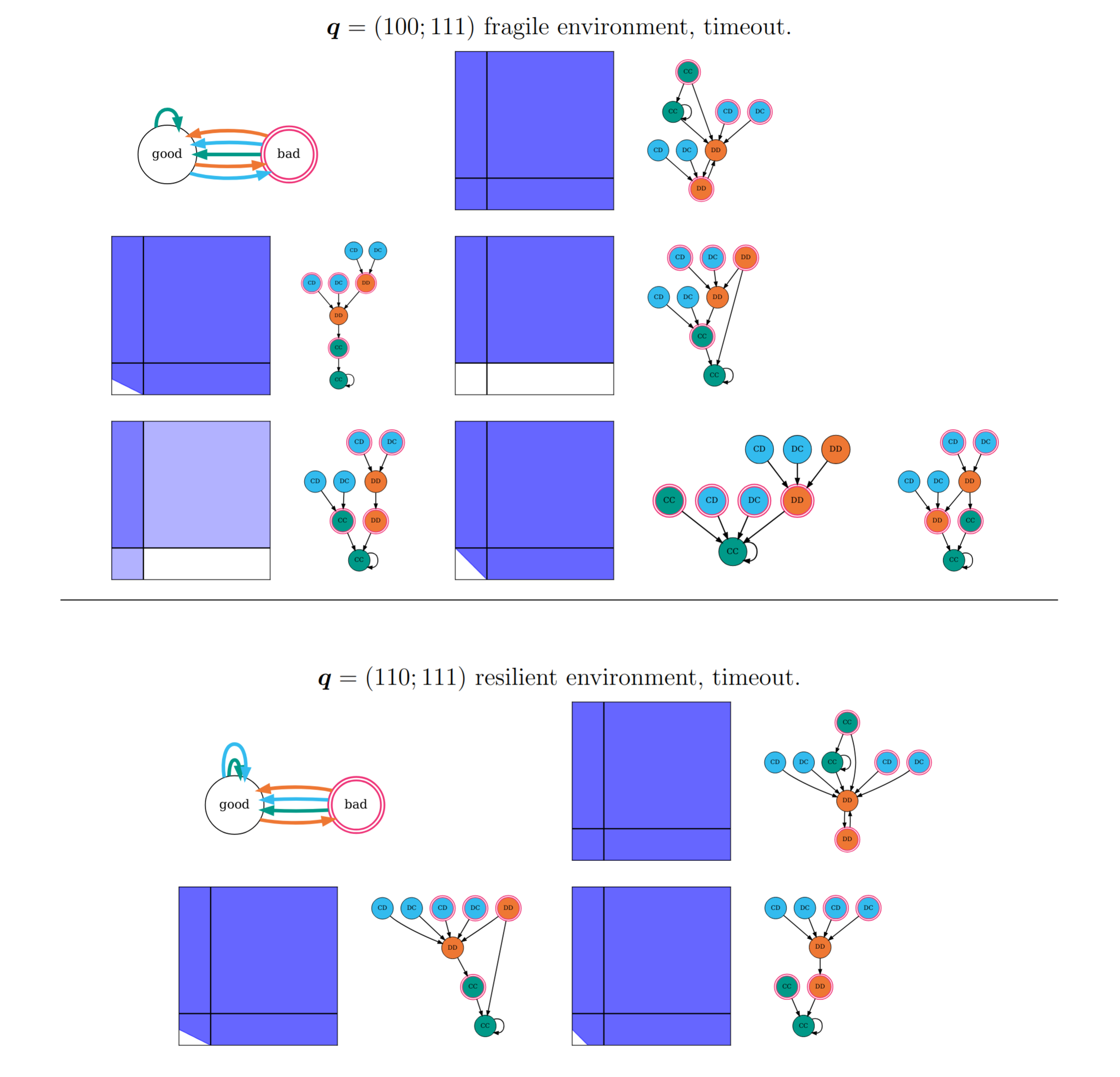
Figure 6. SPNE in timeout environments. From left to right, top to bottom, the \(\boldsymbol{p}\)-groups in the fragile environment are -000-000, 1000-001, 100--111, 1111-000 or 1001-00-, and 1001-110; and in the resilient environment are -000---0, 100----1, and 1001---0.

A strategy that defects in the bad environment when the previous action was DD is only ever a potential SPNE in the timeout environment. The strategy with the weakest necessary condition is such a strategy, and it occurs in the resilient environment.

In the Github repository, I also have results for \(\boldsymbol{q} = (1, -, 0; 1, 0, 1)\). I call this a ‘strange return’ because the bad environment improves when both players defect. Perhaps unsurprisingly, some of the strategies and conditions it finds are quite different from those above, and we can visualise those results similar to the ‘sensible’ environment above and puzzle over what they mean.

References

Kleshnina, M., Hilbe, C., Šimsa, Š., Chatterjee, K. and Nowak, M.A., 2023. The effect of environmental information on evolution of cooperation in stochastic games. Nature Communications, 14(1), p.4153.