Example numerical analysis of replicator dynamics with more than 2 strategies
Recently, I set a task for a student to use Python to analyse the replicator dynamics of a game with three strategies, including using the Jacobian to determine the stability of the steady state. The purpose of this blog post is to share the solution in case that’s useful to someone.
The game
For this task, we will consider the replicator dynamics of a 2-player game with 3 strategies.
Recall the general equation for the replicator dynamics is
\[\begin{equation} \dot{p}_i = p_i (f_i - \bar{f}) \end{equation}\]where \(p_i\) is proportion of \(i\)-strategists in the population, \(f_i\) is fitness effect of strategy \(i\), and \(\bar{f}\) is the average fitness in the population.
The fitness effect is the expected payoff
\[\begin{equation} f_i = \sum_j p_j \pi(i \mid j) \end{equation}\]where \(\pi(i \mid j)\) is the payoff to an \(i\)-strategist who has been paired against a \(j\)-strategist. The average fitness
\[\begin{equation} \bar{f} = \sum_j f_j p_j. \end{equation}\]For this example, the payoffs are given by the matrix
\[\begin{equation} \pi = \begin{pmatrix} 0 & 1 & 4 \\ 1 & 4 & 0 \\ -1 & 6 & 2 \\ \end{pmatrix}, \end{equation}\]where \(\pi(i \mid j)\) is given by element \(\pi_{i,j}\). For example, when strategy 1 plays against strategy 2, strategy 1 receives payoff 1; when strategy 1 plays against strategy 3, strategy 1 receives payoff 4; and so on. This example is taken from Ohtsuki et. al. (2006).
Plot the dynamics
To gain an intuition for the dynamics, we will first plot them.
Marvin Böttcher has written a handy utility for plotting the dynamics of a 3-strategy game on a simplex called egtsimplex. It can be downloaded from the Github repository here: https://github.com/marvinboe/egtsimplex. The repository includes an example that we can look at to see how it works.
First, we need to create a function that defines the dynamics and returns \(\dot{\boldsymbol{p}}\).
def calc_dotps(pis, t):

    # matrix of payoffs between R1, R2, and R3
    payoffs = [
            [ 0,  1,  4],
            [ 1,  4,  0],
            [-1,  6,  2]
            ]

    # replicator dynamics: \dot{p}_i = p_i (f_i - \bar{f})
    # where p_i is proportion of i in the population
    #       f_i is fitness effect of strategy i
    #       f_i = \sum_j p_j pay(i|j) where pay(i|j) is the payoff to i playing against j
    #       \bar{f} is the average fitness in the population
    #       \bar{f} = \sum_j f_j p_j

    # calculate the fitness of each strategy in the population

    fis = list()
    for i in range(3):

        fi = 0
        for j in range(3):

            fi += payoffs[i][j]*pis[j]

        fis.append(fi)

    # average fitness in the population
    fbar = sum(fis[j]*pis[j] for j in range(3))

    # calculate the derivatives
    dotps = [pis[i]*(fis[i]-fbar) for i in range(3)]

    return dotps
Above, I chose to define each fitness effect in a for-loop to be as explict as possible about the connection to the equations above.
To plot the dynamics, we create a simplex_dynamics object called dynamics, and use the method plot_simplex():
import egtsimplex
import matplotlib.pyplot as plt

dynamics = egtsimplex.simplex_dynamics(calc_dotps)

fig,ax = plt.subplots()
dynamics.plot_simplex(ax, typelabels=['R1', 'R2', 'R3'])
plt.show()
That produces a nice graph like the one below.
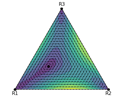
Replicator dynamics on the simplex produced using egtsimplex by Marvin Böttcher
In the process of finding the dynamics, egtsimplex stored the fixed points it found…
fp_xy = dynamics.fixpoints
fp_xy

array([[ 1.00000000e+00, -6.69773909e-14],
       [ 5.00000000e-01,  8.66025404e-01],
       [ 3.57142857e-01,  2.47435830e-01],
       [-3.01051047e-13, -1.99845407e-13],
       [-4.18950369e-15, -2.21083405e-15],
       [ 5.76254503e-14,  3.29021429e-14]])
… however, these are in \((x,y)\) coordinates for plotting.
To get the barycentric coordinates, i.e., the actual quanties of \(p_1\), \(p_2\), and \(p_3\),
we can use the xy2ba() method
fp_ba = [dynamics.xy2ba(x, y) for x, y in fp_xy]
fp_ba

[array([ 2.62163913e-14,  1.00000000e+00, -7.72715225e-14]),
 array([3.31994121e-14, 3.74364097e-18, 1.00000000e+00]),
 array([0.5       , 0.21428571, 0.28571429]),
 array([ 1.00000000e+00, -1.85694097e-13, -2.30639537e-13]),
 array([ 1.00000000e+00, -2.94854279e-15, -2.60257234e-15]),
 array([1.0000000e+00, 3.8651550e-14, 3.8064861e-14])]
The interior steady state is the 3rd one in fp_ba above.
We can already tell from the plot there are oscillatory dynamics,
but it’s not immediately obvious whether the interior steady state is an attractor, repellor, or neutral.
Let’s try plotting a trajectory that starts nearby.
To plot a trajectory, I’ll use solve_ivp with the LSODA method.
I know that \(\sum_j p_j = 1\), so I’ll write a lambda function that takes into account that constraint
and reduce the number of state variables from 3 to 2.
from scipy.integrate import solve_ivp
import numpy as np

# a function that accepts t and the population proportions for the first
# two variables and returns the dv/dt for the first two variables
fnc = lambda t, p: calc_dotps([p[0], p[1], 1-p[0]-p[1]], t)[:2]

# numerically integrate the dynamics
sol = solve_ivp(fnc, [0, 50], [0.5, 0.2], method='LSODA')

# the solution is stored in y
pt = sol.y.T

# look at the first 10 points
pt[:10]

array([[0.5       , 0.2       ],
       [0.5036369 , 0.19880293],
       [0.50716848, 0.19788863],
       [0.5138994 , 0.196637  ],
       [0.51973676, 0.19656723],
       [0.52426076, 0.19769877],
       [0.52731171, 0.20026023],
       [0.52808714, 0.20405974],
       [0.52646399, 0.2088587 ],
       [0.52363774, 0.21300196]])
To add the trajectory to the plot,
we will need to revert pt above from a 2-dimensional to 3-dimensional system,
and then convert the 3-dimensional barycentric coordinates to \((x,y)\) for plotting.
traj_xy = list()

for p1, p2 in pt:

    p3 = 1 - p1 - p2
    traj_xy.append(list(dynamics.ba2xy([p1, p2, p3])))

traj_x, traj_y = zip(*traj_xy)

# plot the simplex dynamics again and put the trajectory on top in red
fig,ax = plt.subplots()
dynamics.plot_simplex(ax, typelabels=['R1', 'R2', 'R3'])
ax.scatter([traj_x[0]], [traj_y[0]], color='red')
ax.plot(traj_x, traj_y, color='red')
plt.show()
That produces the figure below, which suggests that the interior steady state is unstable.
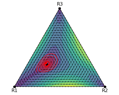
A trajectory of the replicator dynamics (start point marked with dot)
Use the eigenvalues of the Jacobian matrix to assess the stability of the interior steady state
Ohtsuki et al. (2006) determined the eigenvalues of the Jacobian matrix analytically, but let’s use this example to learn how we would do so numerically.
First, we need to get an expression for each element of the Jacobian matrix.
Recall the replicator dynamics:
\[\begin{equation} \dot{p}_i = p_i (f_i - \bar{f}) \end{equation}\]Each element of the Jacobian matrix
\[\begin{equation} J_{i,k} = \left. \frac{\partial \dot{p}_i}{\partial p_k} \right|_{\boldsymbol{p}^*} = \left. [f_i - \overline{f}] \right|_{\boldsymbol{p}^*} + p_i^* \left( \left. \frac{\partial f_i}{\partial p_k} \right|_{\boldsymbol{p}^*} - \left. \frac{\partial \overline{f}}{\partial p_k} \right|_{\boldsymbol{p}^*} \right) \end{equation}\]At \(\boldsymbol{p}^*\), \(f_i = \overline{f}\), so
\[\begin{equation} J_{i,k} = p_i^* \left( \left. \frac{\partial f_i}{\partial p_k} \right|_{\boldsymbol{p}^*} - \left. \frac{\partial \overline{f}}{\partial p_k} \right|_{\boldsymbol{p}^*} \right) \tag{1} \end{equation}\]Write the expression for each derivative individually, replacing the last variable: \(p_m = 1 - \sum_{j=1}^{m-1} p_j\).
To get the left-hand term in the Jacobian element, start with
\[\begin{align} f_i &= \sum_{j=1}^m p_j \pi(i \mid j) \\ &= \left[ \sum_{j=1}^{m-1} p_j \pi(i \mid j) \right] + \pi(i \mid m) \left[ 1 - \sum_{j=1}^{m-1} p_j \right] \\ &=\left[ \sum_{j=1}^{m-1} p_j [\pi(i \mid j) - \pi(i \mid m)] \right] + \pi(i \mid m) \end{align}\]Therefore:
\[\begin{equation} \left. \frac{\partial f_i}{\partial p_k} \right|_{\boldsymbol{p}^*} = \pi(i \mid k) - \pi(i \mid m) \tag{left-hand term of (1)} \end{equation}\]For the right-hand term in the Jacobian element, split the population average fitness effect into three terms
\[\begin{equation} \overline{f} = \sum_j p_j f_j = \left[ \sum_{j=1, j\neq k}^{m-1} p_j f_j \right] + p_k f_k + p_m f_m \end{equation}\]and take the derivatives of each term separately.
The first term:
\[\begin{align} \left. \frac{\partial}{\partial p_k} \left[ \sum_{j=1, j \neq k}^{m-1} p_j f_j \right] \right|_{\boldsymbol{p}^*} &= \sum_{j=1, j \neq k}^{m-1} p_j^* \left. \frac{\partial f_j}{\partial p_k} \right|_{\boldsymbol{p}^*} \\ &=\sum_{j=1, j \neq k}^{m-1} p_j^* [\pi(j \mid k) - \pi(j \mid m)] \end{align}\]The second term:
\[\begin{align} \left. \frac{\partial \left[ p_k f_k \right]}{\partial p_k} \right|_{\boldsymbol{p}^*} &= \left. f_k \right|_{\boldsymbol{p}^*} + p_k^* \left. \frac{\partial f_k}{\partial p_k} \right|_{\boldsymbol{p}^*} \\ &= \left[ \sum_{j=1}^m p^*_j \pi(k \mid j) \right] + p_k^* [\pi(k \mid k) - \pi(k \mid m)] \end{align}\]The third term:
\[\begin{align} \left. \frac{\partial \left[ p_m f_m \right]}{\partial p_k} \right|_{\boldsymbol{p}^*} &= \left. \frac{\partial }{\partial p_k} \left[1-\sum_{j=1}^{m-1} p_j \right] \right|_{\boldsymbol{p}^*} \left. f_m \right|_{\boldsymbol{p}^*} + p_m^* \left. \frac{\partial f_m}{\partial p_k} \right|_{\boldsymbol{p}^*} \\ &= - \left[ \sum_{j=1}^m p_j^* \pi(m \mid j) \right] + p_m^* [\pi(m \mid k) - \pi(m \mid m)] \end{align}\]So summing them together to get the right-hand term in the Jacobian element:
\[\begin{equation} \left. \frac{\partial \overline{f}}{\partial p_k} \right|_{\boldsymbol{p}^*} = \sum_{j=1}^m p_j^* [ \pi(j \mid k) - \pi(j \mid m) + \pi(k \mid j) - \pi(m \mid j) ] \tag{right-hand term of (1)} \end{equation}\]Let’s now code the Jacobian.
First, code the payoffs so \(\pi(j \mid k) =\) pays[j][k]
and the interior steady state \(p_j^* =\) ps[j].
pays = [ [ 0,  1,  4], [ 1,  4,  0], [-1,  6,  2] ]
ps = fp_ba_tidy[2] # recall the interior steady state was the third element
Code the right-hand term of (1), \(\begin{equation} \left. \frac{\partial \overline{f}}{\partial p_k} \right|_{\boldsymbol{p}^*} \end{equation}\)
m = 2 # because Python counts indices 0, 1, 2 instead of 1, 2, 3
dfbar_dps = [ sum(ps[j]*(pays[j][k]-pays[j][m] + pays[k][j] - pays[m][j]) for j in range(3)) for k in range(2)]
Code the full \(J_{i,k}\) in (1)
J = np.array([ [ps[i]*(pays[i][k] - pays[i][m] - dfbar_dps[k]) for i in range(2)] for k in range(2) ])We find that the Jacobian matrix is
J

array([[-0.67857143,  0.78061224],
       [-1.75      ,  0.75      ]])
and its eigenvalues
w, v = np.linalg.eig(J) # w are the eigenvalues, v are the eigenvectors
w

array([0.03571429+0.92513099j, 0.03571429-0.92513099j])
The maximum real part is positive, so the interior steady state is unstable.
References
Ohtsuki, H., & Nowak, M. A. (2006). The replicator equation on graphs. Journal of Theoretical Biology, 243(1), 86-97.