Lab meeting about threshold games
Last month, I chose a paper by Kris De Jaegher in Scientific Reports for our weekly lab-meeting discussion. We used the paper to teach ourselves about threshold games, and the purpose of this blog post is to summarise the things we learnt.
Replicator dynamics revision
De Jaegher used the replicator dynamics approach. Replicator dynamics assumes a well-mixed, infinitely large population of players that reproduces asexually, where the number of offspring they produce depends upon the payoff they receive from a game-theoretic ‘game’, as illustrated below:–
Replicator dynamics animation, created by HowieKor (Creative Commons)
We start with a population of \(n\) individuals with different game strategies. Individuals are randomly selected to form groups and play the game. The payoff from the game determines how many offspring they have. Offspring inherit the strategies of their parents (clonal reproduction), and the cycle repeats.
Let’s rederive the dynamics. The number of individuals pursuing strategy \(i\) changes according to
\[\frac{dn_i}{dt} = \dot{n_i} = n_i (\beta + f_i),\]where \(\beta\) is the background reproduction rate (apart from the game’s effect), and \(f_i\) is the fitness effect of playing strategy \(i\).
Denote the proportion of \(i\)-strategists in the population
\[p_i = \frac{n_i}{N}\]where \(N\) is the total population size.
We want to know \(\frac{dp_i}{dt}\). Rearrange the \(p_i\) definition and take the derivatives
\[n_i = p_i N\] \[\dot{n_i} = p_i \dot{N} + \dot{p_i} N\] \[\dot{p} = \frac{1}{N} (\dot{n_i} - p_i \dot{N})\]So we need to sort out \(\dot{N}\)
\[\begin{align} \dot{N} &= \sum_i \dot{n_i} \\ &= \beta \sum_i n_i + \sum_i f_i n_i \\ &= \beta N + N \sum_i f_i \frac{n_i}{N} \\ &= \beta N + N \sum_i f_i p_i \\ \dot{N} &= N (\beta +\bar{f}) \\ \end{align}\]Substitute our equations for \(\dot{N}\) and \(\dot{n_i}\) into the equation for \(\dot{p_i}\), and we obtain the dynamics of strategy proportions
\[\frac{dp_i}{dt} = \dot{p} = p_i (f_i - \bar{f})\]In the De Jaegher paper, players face the binary choice of cooperating or defecting. Denote cooperators and defectors by C and D, respectively, and define \(p = p_C = 1-p_D\). Then the equation governing the dynamics simplifies to
\[\begin{align} \dot{p} &= p \, (f_C - [p f_C + (1-p) f_D]) \\ \dot{p} &= p (1-p) (f_C - f_D) \end{align}\]Threshold game
In the threshold game, a group is formed with \(n\) players (different to \(n\)) above, and if the group contains \(k\) or more cooperators, then they provide a benefit \(b\). The benefit \(b\) is received by all group members regardless of whether that member was a cooperator or defector
\[b_i = \begin{cases} b &\text{if } i >= k \text{ (threshold met)}\\ 0 &\text{otherwise (threshold not met)} \end{cases}\]Throughout their paper, they have normalised \(b=1\).
import numpy as np
from scipy.special import binom
import matplotlib.pyplot as plt
from scipy.optimize import brentq

b = lambda x, k: 1 if x >= k else 0

k = 5
xV = list(range(7+1))
bV = [b(x, k) for x in xV]

plt.title('7 player game w. threshold $k=5$')
plt.plot(xV, bV, '-o', color='blue')
plt.xlabel('no. cooperators in group')
plt.ylabel('benefit $b$')
plt.xticks(range(7+1))
plt.show()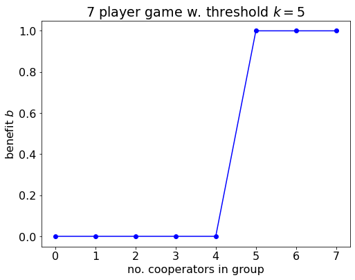
Benefit provided to each player in the threshold game as a function of the number of cooperators in the group.
Everyone receives the benefit, but only cooperators pay the cost \(c\). So the total payoff to cooperators is
\[\text{cooperator payoff} = \begin{cases} b - c & \text{if threshold met,} \\ -c & \text{if threshold not met.} \end{cases}\]and defectors receive
\[\text{defector payoff} = \begin{cases} b & \text{if threshold met,} \\ 0 & \text{if threshold not met.} \end{cases}\]Defectors always do better than cooperators.
n = 7
k = 5
c = 0.4

xV = list(range(n+1))

# payoffs
pay_C = [ b(x, k) - c for x in xV[1:] ]
pay_D = [ b(x, k) for x in xV[:-1] ]

plt.plot(xV[1:], pay_C, '-o', color='blue', label='cooperators')
plt.plot(xV[:-1], pay_D, '-o', color='red', label='defectors')

plt.title('7 player game w. threshold $k=5$')
plt.legend(loc='best')
plt.xlabel('no. of cooperators in group')
plt.ylabel('total payoff')
plt.xticks(range(n+1))
plt.show()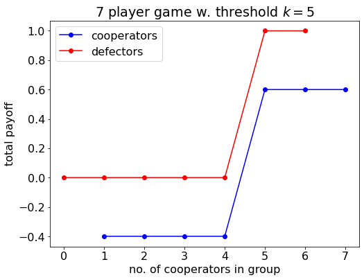
Payoff to cooperators and defectors in the threshold game as a function of the number of cooperators in the group.
Fitness effects
The payoffs above tell us about what happens in a particular game with a particular number of cooperators and defectors, but we need the fitness effects of being a cooperator and defector, \(f_C\) and \(f_D\), which are averaged over all the games played.
The replicator dynamics assumes that groups are formed randomly from an infinite population, so the make-up of the other players is binomially distributed. Therefore, the fitness effect is the sum of the payoffs from each game multiplied by the probability that the player will end up in that game
\[f_C(p) = \sum_{i=0}^{n-1} \underbrace{ {n-1 \choose i} p^i (1-p)^{n-1-i}}_{\text{Pr grouped with $i$ cooperators}} \: b_{i+1} - c,\] \[f_D(p) = \sum_{i=0}^{n-1} \underbrace{ {n-1 \choose i} p^i (1-p)^{n-1-i}}_{\text{Pr grouped with $i$ cooperators}} \: b_{i}.\]f_c = lambda p, c, k, n: sum(binom(n-1, l) * p**l * (1-p)**(n-1-l) * b(l+1, k) for l in range(n)) - c
f_d = lambda p, c, k, n: sum(binom(n-1, l) * p**l * (1-p)**(n-1-l) * b(l, k) for l in range(n))Pivot probability
The pivot probability is the probability that a player will end up in a game where \(k-1\) of the other \(n-1\) players is a cooperator
\[\pi_k = {n-1 \choose k-1} p^{k-1} (1-p)^{n-k}.\]pi_k_fnc = lambda p, k, n: binom(n-1, k-1) * p**(k-1) * (1-p)**(n-k)
n = 7
k = 5
c = 0.4
# y is the number of the other n-1 players who are cooperators
yV = list(range(n))
# payoffs
pay_C = [ b(y+1, k) - c for y in yV ]
pay_D = [ b(y, k) for y in yV ]
plt.plot(yV, pay_C, '-o', color='blue', label='cooperators')
plt.plot(yV, pay_D, '-o', color='red', label='defectors')
# show the pivot
plt.annotate(text='', xy=(4, 0), xytext=(4, 1-c), arrowprops=dict(arrowstyle='<->', linewidth=4))
plt.title('7 player game w. threshold $k=5$')
plt.legend(loc='best')
plt.xlabel('no. of cooperators among $n-1$ other players')
plt.ylabel('total payoff')
plt.xticks(range(7))
plt.show()Why is the pivot probability significant? First, consider just a single game, and imagine I know that I am the pivotal player. If I am a cooperator, then it is in my interests to remain a cooperator because if I switch then I will reduce my own payoff. If I am defector and I have the option of switching strategies, I would want to switch to cooperate.
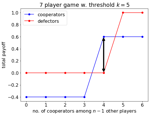
Payoff to cooperators and defectors in the threshold game as a function of the number of cooperators among the other members of the group. If I am the pivotal player, then it is in my interests to cooperate (marked with an arrow).
We can also intuit that, if the probability that I will end up in a game where I am the pivotal player is high, then assuming I have a fixed strategy that I play all the time, it might be in my interests to be a cooperator… We’ll return to this point soon.
First example of the threshold game
Let’s just plot an example to start with to get a sense of the dynamics. Recall
\[\dot{p} = p (1-p) (f_C - f_D)\]where \(f_C\) and \(f_D\) defined in the paper. Let us plot this.
# dynamics equation
delta_p = lambda p, c, k, n: p*(1-p)*(f_c(p, c, k, n) - f_d(p, c, k, n))

# some parameter values
n = 7
k = 5
c = 0.3

# how Delta p changes with p
pV = np.linspace(0, 1, 60)
delta_pV = [ delta_p(p, c, k, n) for p in pV ]
plt.plot(pV, delta_pV, color='blue', label=r'$\frac{dp}{dt}$')

# solve for stable steady state

# the p-value at the peak (I'll explain this bit later)
p_hat_fnc = lambda k, n: (k-1)/(n-1)
p_hat = p_hat_fnc(k, n)
eql0 = lambda p: pi_k_fnc(p, k, n) - c
p_s = brentq(eql0, p_hat, 0.9)
plt.scatter([p_s], [0], s=50, color='black')

# also plot defector steady state
plt.scatter([0], [0], s=50, color='black')

# show changes with arrows
y = 0.01
p_u = brentq(eql0, p_hat, 0.1) # solve for unstable steady state
plt.annotate(text='', xy=(0, y), xytext=(p_u, y), arrowprops=dict(arrowstyle='->', linewidth=2))
plt.annotate(text='', xy=(p_u, y), xytext=(p_s, y), arrowprops=dict(arrowstyle='<-', linewidth=2))
plt.annotate(text='', xy=(p_s, y), xytext=(1, y), arrowprops=dict(arrowstyle='->', linewidth=2))

# decorate plot
plt.title('$k=5$, $n=7$')
plt.axhline(0, color='black')
plt.xlabel('propn cooperators $p$')
plt.ylabel(r'change in coops $\frac{dp}{dt}$')
plt.legend(loc='lower right')
plt.ylim((-0.06, 0.02))
plt.show()
In the figure below, we find that the all-defector population is an evolutionarily stable steady state, and the all-cooperation population is unstable. There is also an evolutionarily stable state with a mix of cooperators and defectors (at \(p^{\star} = 0.746\)).
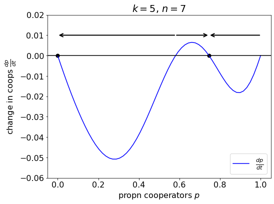
How the change in the proportion of cooperators varies with the current proportion of cooperators (p). There are 2 stable steady states (marked with a solid dot) and two unstable steady states. The arrows indicate the direction in which the population will evolve given its current (p) value.
We can also see some of this directly by inspecting the equation for the dynamics. Recall
\[\frac{dp}{dt} = p (1-p) (f_C(p) - f_D(p)).\]Steady states occur when \(\frac{dp}{dt} =0\), so there are two trivial steady states
\[p = 0,\]and
\[p = 1.\]and any interior steady states solve
\[0 = f_C(p) - f_D(p).\]Let’s focus on these interior steady states. Recall
\[f_C(p) = \sum_{i=0}^{n-1} { n-1 \choose i } p^i (1-p)^{n-1-i} b_{i+1} - c,\]and
\[f_D(p) = \sum_{i=0}^{n-1} { n-1 \choose i } p^i (1-p)^{n-1-i} b_i,\]but the \(b_i\) values are only 1 when \(i >=k\), otherwise 0. Therefore, we can simplify
\[f_C(p) - f_D(p) = \underbrace{ {n-1 \choose k-1} p^{k-1} (1-p)^{n-k}}_{\pi_k(p)} - c,\]and notice that the pivot probability is in it.
In summary, the dynamics are
\[\frac{dp}{dt} = p \, (1-p) \, \overbrace{ \underbrace{ {n-1 \choose k-1} p^{k-1} (1-p)^{n-k} }_{\pi_k(p)} - c}^{f_C(p) - f_D(p)}\]Let’s plot just the function that solves the interior steady states
\[\pi_k(p) - c = 0.\]# our \pi_k(p) - c = 0 function to solve
Delta_f = lambda p, c, k, n: pi_k_fnc(p, k, n) - c
# some parameter values
n = 7
k = 5
c = 0.3
# how the delta f function changes with p
Delta_fV = [ Delta_f(p, c, k, n) for p in pV ]
plt.plot(pV, Delta_fV, color='blue', label=r'$f_C - f_D$')
# the p-value at the peak (see further below for explanation)
p_hat = p_hat_fnc(k, n)
# solve for stable steady state
eql0 = lambda p: pi_k_fnc(p, k, n) - c
p_s = brentq(eql0, p_hat, 0.9)
plt.scatter([p_s], [0], s=50, color='black', label='where $\pi_k(p)-c=0$')
# decorate plot
plt.title('$k=5$, $n=7$')
plt.axhline(0, color='black')
plt.xlabel('propn cooperators $p$')
plt.ylabel(r'$f_C(p) - f_D(p)$')
plt.legend(loc='best')
plt.show()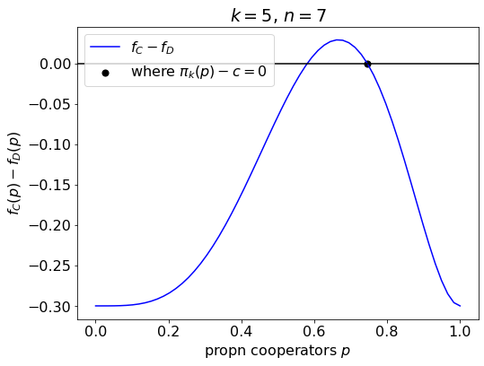
How the difference in fitness effects changes with the proportion of cooperators. This function also isolates the interior steady states, which solve ( \pi_k(p) - c = 0 ) (stable steady state shown with a solid dot).
The peak
De Jaegher found that, when \(1 < k < n\), both \(f_C - f_D\) and \(\pi_k\) have a peak at \(\hat{p} = \frac{k-1}{n-1}\). They found this by taking advantage of the fact that the function is unimodal, and finding when the derivative was 0.
\[f_C(p) - f_D(p) = {n-1 \choose k-1} p^{k-1} (1-p)^{n-k} - c,\]so
\[\frac{d(f_C(p) - f_D(p))}{dp} = {n-1 \choose k-1} (1-p)^{n-k-1} p^{k-2} \bigl( (k-1)(1-p) + (k-n) p \bigr).\]The peak is located where \(\frac{d(f_C(p) - f_D(p))}{dp} = 0\) that is
\[0 = (k-1)(1-\hat{p}) + (k-n) \hat{p},\]which gives the peak location
\[\hat{p} = \frac{k-1}{n-1}.\]Because \(f_C - f_D\) and \(\pi_k\) differ only by a constant, this point is also the location of the peak of the pivot probability function.
# some parameter values
n = 7
k = 5
c = 0.3

# how the gain function changes with p
Delta_fV = [ Delta_f(p, c, k, n) for p in pV ]
plt.plot(pV, Delta_fV, color='blue', label=r'$f_C - f_D$')

# the p-value at the peak
p_hat = p_hat_fnc(k, n)
plt.axvline(p_hat, color='black', ls='dashed', label='peak $\hat{p}$')

# solve for steady state
eql0 = lambda p: pi_k_fnc(p, k, n) - c
p_s = brentq(eql0, p_hat, 0.9)
plt.scatter([p_s], [0], s=50, color='black')

# decorate plot
plt.title('$k=5$, $n=7$')
plt.axhline(0, color='black')
plt.xlabel('propn cooperators $p$')
plt.ylabel(r'$f_C(p) - f_D(p)$')
plt.legend(loc='best')
plt.show()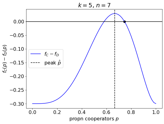
Example showing the location fo the peak.
Knowing where this peak is and whether it is above or below the line tells us about the dynamics, as will become clearer in the examples below.
Examples for Result 1
Below, we’ll go through examples for each of the cases in Result 1.
# keep group-size parameter value constant
n = 7

# grid size for plotting
pV = np.linspace(0, 1, 60)
When \(k=1\)
For the minimal threshold \(k = 1\), the game has a unique interior fxed point where a fraction \(p_1^{\text{II}} = 1-c^{1/(n-1}\) of players cooperates (Volunteer’s Dilemma).
k = 1

# how Delta p changes with p
delta_pV = [ delta_p(p, c, k, n) for p in pV ]
plt.plot(pV, delta_pV, color='blue', label=r'$\frac{dp}{dt}$')

# fixed point
p_s = 1-c**(1/(n-1))
plt.scatter([p_s], [0], s=50, color='black', label='$p_1^{II}$')

# decorate plot
plt.title('$k=1$')
plt.axhline(0, color='black')
plt.xlabel('propn cooperators $p$')
plt.ylabel(r'change in coops $\frac{dp}{dt}$')
plt.legend(loc='best')
plt.show()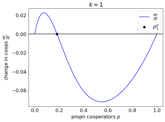
Example dynamics for the Volunteer’s Dilemma.
When \(1 < k < n\)
Low cost
When participation costs are small (\(c < \bar{c}_k\)), the game both has a fixed point where all players defect (\(p = 0\)) and a stable fixed point \(p_k^{\text{II}}\), which is implicitly given by \(\pi_k(p_k^{\text{II}}) = c\).
k = 5
c = 0.3

# how Delta p changes with p
delta_pV = [ delta_p(p, c, k, n) for p in pV ]
plt.plot(pV, delta_pV, color='blue', label=r'$\frac{dp}{dt}$')

# the p-value at the peak
p_hat = p_hat_fnc(k, n)

# the pivot probability at the p-value at the peak
c_bar = pi_k_fnc(p_hat, k, n)

# solve for steady state
eql0 = lambda p: pi_k_fnc(p, k, n) - c
p_s = brentq(eql0, p_hat, 0.9)
plt.scatter([p_s], [0], s=50, color='black', label='$p_k^{II}$')

# also plot defector ss
plt.scatter([0], [0], s=50, color='black')

# decorate plot
plt.title('$k=5$, ' + str(c) + ' = $c < c_k$ = ' + str(int(1000*c_bar)/1000))
plt.axhline(0, color='black')
plt.xlabel('propn cooperators $p$')
plt.ylabel(r'change in coops $\frac{dp}{dt}$')
plt.legend(loc='best')
plt.show()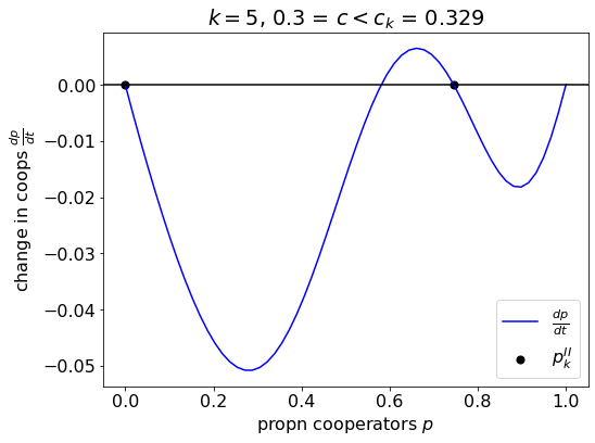
Example dynamics for the Hybrid Game.
High cost
When participation costs are high, \(c > \bar{c}_k\), the game has a unique stable fixed point where all players defect (\(p = 0\)).
c = 0.35

# how Delta p changes with p
delta_pV = [ delta_p(p, c, k, n) for p in pV ]
plt.plot(pV, delta_pV, color='blue', label=r'$\frac{dp}{dt}$')

# the p-value at the peak
p_hat = p_hat_fnc(k, n)

# plot defector ss
plt.scatter([0], [0], s=50, color='black')

# decorate plot
plt.title('$k=5$, ' + str(c) + ' = $c > c_k$ = ' + str(int(1000*c_bar)/1000))
plt.axhline(0, color='black')
plt.xlabel('propn cooperators $p$')
plt.ylabel(r'change in coops $\frac{dp}{dt}$')
plt.legend(loc='best')
plt.show()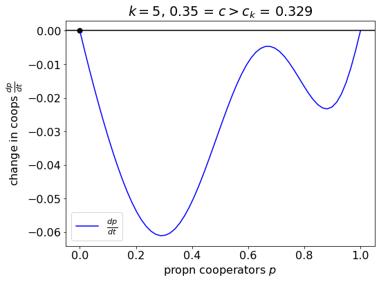
Example dynamics for the situation they liken to the Prisoner’s Dilemma.
What’s the significance of this \(\bar{c}_k\) value? Recall
\[f_C(p) - f_D(p) = \underbrace{ {n-1 \choose k-1} p^{k-1} (1-p)^{n-k}}_{\pi_k(p)} - c.\]They’ve defined
\[\bar{c}_k = \pi_k(\hat{p}),\]where \(\hat{p}\) is the probability at the peak. So we know that, if \(\bar{c}_k > c\), the \(f_C - f_D\) line will be above the zero line at the peak and there will be an interior equilibrium, and if \(\bar{c}_k < c\), the peak is below the line and there are no interior equilibria.
When \(k = n\)
Our final case is the maximum threshold, \(k=n\). Here, the game both has a stable steady state where all players defect (\(p = 0\)), and a stable steady state where all players cooperate (\(p = 1\)). The basin of attraction is defined by \(p_n^{\text{I}} = c^{1/(n-1)}\), the unstable interior steady state.
k = n
c = 0.3

# how Delta p changes with p
delta_pV = [ delta_p(p, c, k, n) for p in pV ]
plt.plot(pV, delta_pV, color='blue', label=r'$\frac{dp}{dt}$')

# the pivot probability at the p-value at the peak
pi_k = pi_k_fnc(p_hat, k, n)

# separatrix

# trivial equilibria are steady states
plt.scatter([0], [0], s=50, color='black')
plt.scatter([1], [0], s=50, color='black')

# decorate plot
plt.title('$k=n$')
plt.axhline(0, color='black')
plt.xlabel('propn cooperators $p$')
plt.ylabel(r'change in coops $\frac{dp}{dt}$')
plt.legend(loc='best')
plt.show()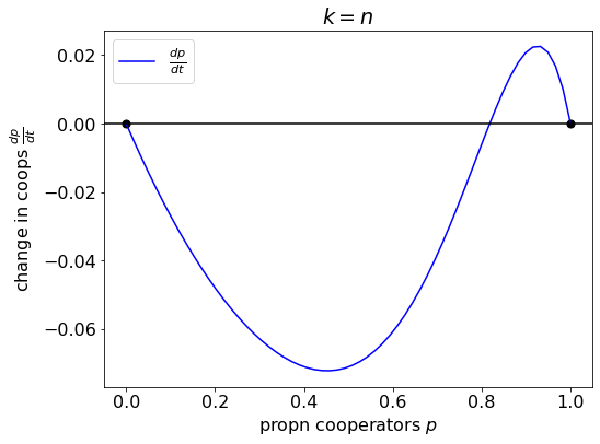
Example dynamics for the situation they liken to a Stag Hunt.
Bringing it all together
We can place each of these examples on De Jaegher’s Fig. 4. The 4 regions of the figure represent four different qualitative regimes for the dynamics (game types).
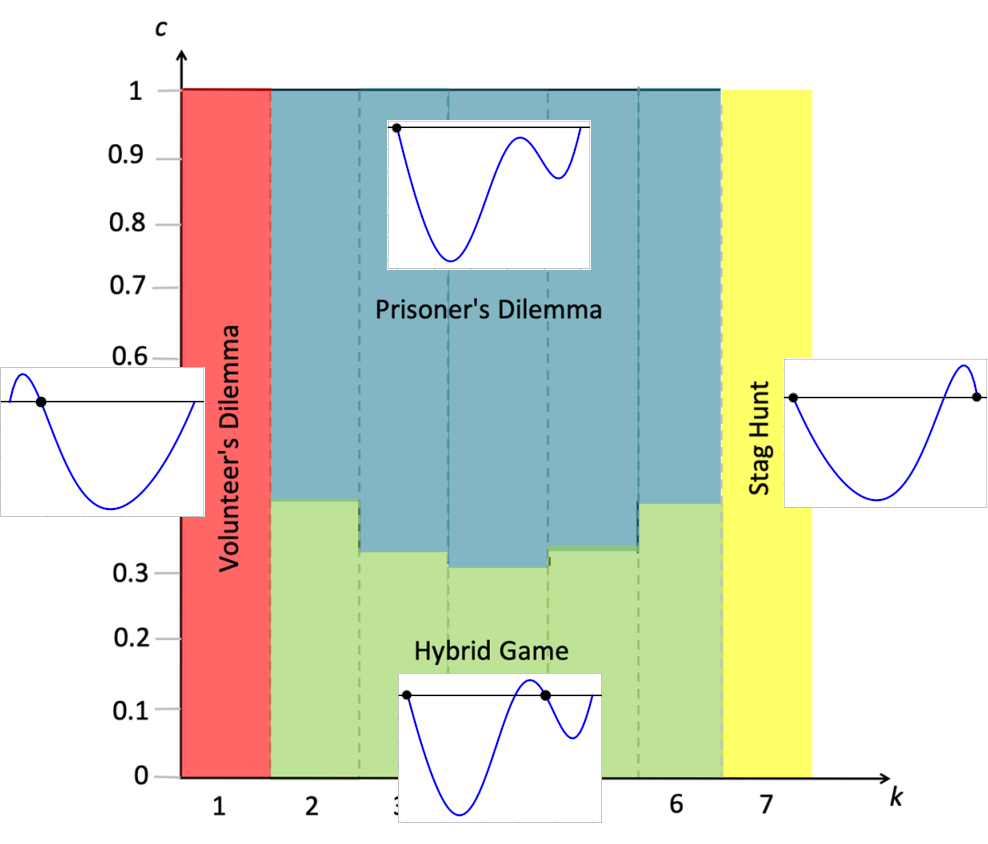
Placing each of our examples onto De Jaegher’s Fig. 4. The four regions reprsent four qualitatively different regimes for the dynamics.
Examples for Result 2
De Jaegher found that the threshold level has a U-shaped efect on the level of cooperation, which can be seen in their Fig. 4 (the shape of the division between the blue and green region). Let’s plot how the dynamics varies with varying threshold level.
n = 7
c = 0.33

for k in range(1, n+1):

    # how Delta p changes with p
    delta_pV = [ delta_p(p, c, k, n) for p in pV ]
    plt.plot(pV, delta_pV, label=str(k))

# decorate plot
plt.title(r'the full $\frac{dp}{dt}$')
plt.axhline(0, color='black')
plt.xlabel('propn cooperators $p$')
plt.ylabel(r'change in coops $\frac{dp}{dt}$')
plt.legend(loc='upper center', title='$k=$', ncol = 7, fontsize='x-small')
plt.ylim((-0.1, 0.06))
plt.show()
Here, we see that cooperation can evolve both for low and for high thresholds, but not for intermediate thresholds. It is perhaps surprising because, intuitively, it seems like a high threshold would be more difficult to obtain.
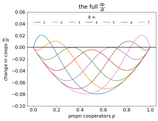
The effect of different threshold levels on the dynamics. In this example, cooperation can evolve if the threshold is low or high, but not for intermediate values.
This U-shape emerges from the pivot probabilities.
n = 7
c = 0.33

for k in range(1, n+1):

    # how Delta p changes with p
    pi_kV = [ pi_k_fnc(p, k, n) for p in pV ]
    plt.plot(pV, pi_kV, label=str(k))

# decorate plot
plt.title('just the $\pi_k$ bit')
plt.axhline(0, color='black')
plt.xlabel('propn cooperators $p$')
plt.ylabel('$\pi_k(p)$')
plt.legend(loc='upper center', title='$k=$', ncol = 7, fontsize='xx-small')
plt.show()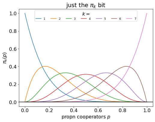
Different threshold levels have a U-shaped effect on the pivot probability.
Group size
De Jaegher discuss the possibility of stabilising a game by changing the group size. If cooperation is more likely to persist at low or high thresholds, then perhaps increasing or decreasing the group size to shift the relative position of the threshold could stabilise cooperation.
It turns out this is true for decreasing the group size, but not for increasing it. Increasing the group size has a negative effect on cooperation.
n = 7
c = 0.33
k = 4

# plot the previous
delta_pV = [ delta_p(p, c, k, n) for p in pV ]
plt.plot(pV, delta_pV, color='black', ls='dashed')

# plot for a range
nV = [4, 5, 6, 8, 12]
for n in nV:

    # how Delta p changes with p
    delta_pV = [ delta_p(p, c, k, n) for p in pV ]
    plt.plot(pV, delta_pV, label=str(n))

# decorate plot
plt.title(r'the full $\frac{dp}{dt}$')
plt.axhline(0, color='black')
plt.xlabel('propn cooperators $p$')
plt.ylabel(r'change in coops $\frac{dp}{dt}$')
plt.legend(loc='upper center', title='$n=$', ncol = 7, fontsize='x-small')
plt.ylim((-0.1, 0.06))
plt.show()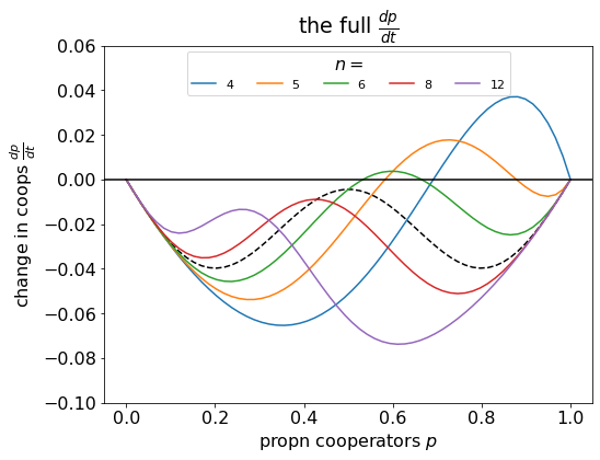
In this example, we have kept the threshold level (k=4) constant, but varied the group size. Decreasing the group size allows the interior steady state, with coexistence of cooperators and defectors, to emerge; but increasing the group size has a negative effect on cooperation.
The reason why is due to the effect of group size on the pivot probability: the larger the group is, the less likely it is for a player to be the pivotal player, and so the lower the benefit of being a cooperator.
n = 7
c = 0.33
k = 4

# plot the previous
pi_kV = [ pi_k_fnc(p, k, n) for p in pV ]
plt.plot(pV, pi_kV, color='black', ls='dashed')

# plot for a range
nV = [4, 5, 6, 8, 12]
for n in nV:

    # how pivot probability changes with p
    pi_kV = [ pi_k_fnc(p, k, n) for p in pV ]
    plt.plot(pV, pi_kV, label=str(n))

# decorate plot
plt.title('just the $\pi_k$ bit')
plt.axhline(0, color='black')
plt.xlabel('propn cooperators $p$')
plt.ylabel('$\pi_k(p)$')
plt.legend(loc='upper center', title='$n=$', ncol = 7, fontsize='xx-small')
plt.show()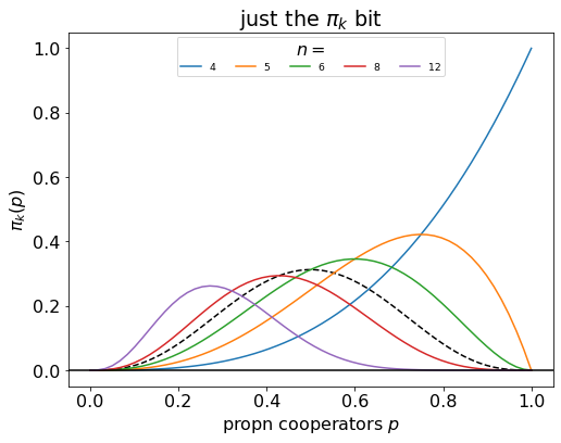
The larger the group size is, the less likely it is that a player is the pivotal player.
References
De Jaegher, K. (2020). High thresholds encouraging the evolution of cooperation in threshold public-good games. Scientific Reports, 10(1), 1-10.