Finding cell neighbours in an ISEA3H global grid in dggridR
In order to model a spatially discretised process on the whole Earth, we need a discrete global grid system (DGGS). Ideally, the DGGS would divide the globe into a tessellation of some regular polygon, analogous to a grid of squares on the plane, where the grid resolution can be increased by further subdivision of the polygon. Another desirable property would be to have equal-distant centres, such as a hexagonal grid, so that the neighbourhood of a grid cell is well defined. Unfortunately, it is not possible to tessellate a sphere with hexagons only, and there are mathematical limits to e.g. the number of points that can be completely regularly distributed on a sphere. As a consequence, finding the ‘best’ DGGS is a research area of its own.
The most popular approach to defining a DGGS is to start with a regular base polyhedron, one of the platonic solids, and then partition its faces into a grid in a hierarchical fashion. Then some method is needed for projecting that grid on the solid onto a spherical surface, with the goal of preserving as far as possible the desirable properties of the grid, such as the equal areas or regular angles and distances between centre points. Because there are many possible options for each of the design choices (base polyhedron, its orientation, grid shape, etc.), there are quite a number of different DGGS available, each with their own strengths and weaknesses (Sahr et al., 2003). Therefore, I decided to work with the most popular DGGS available, as it will probably be the DGGS that offers the best compromise between desirable properties, and it will have the most software and support available for it.
The Icosahedral Snyder Equal Area Aperture 3 Hexagonal Grid, or ISEA3H (Fig. 1) appears to be the most popular DGGS (Mocnik, 2019). Its base polyhedron is the icosahedron, with its triangular faces partitioned into hexagons. Because each vertex of the icosahedron is the meeting of 5 triangles, the grid shape at each vertex is necessarily a pentagon. Therefore the grid contains 12 pentagons in total, regardless of the grid resolution, with area 5/6 the area of the hexagons.
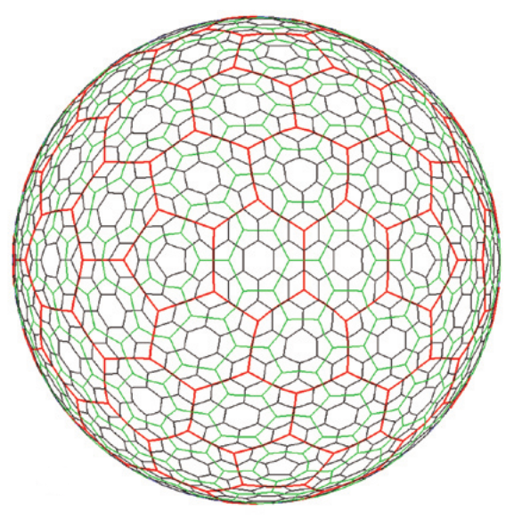
Figure 1. The ISEA3H global grid at resolutions 2 (red), 3 (green), and 4 (purple), taken from Sahr et al. (2003).
‘Aperture 3’ refers to the way in which refinements of the hexagons are performed, with the area of each hexagon decreasing by 1/3 at each increasing resolution (Fig. 2). Aperture 3 is preferred because it is lower than the (only?) alternative, aperture 4. In aperture 3, the refinements of the grid at each resolution cause the hexagons to alternate between two orientations: point at top and edge at top. Consequently, for each even-numbered resolution (e.g. resolution 2, blue) the triangle edge runs through the hexagon centres (‘Class I’), whereas for each odd-numbered resolution (e.g. resolution 3, red) the triangle edge alternates between being aligned with a centre or an edge of a hexagon cell (‘Class II’). This creates complications for an axes-based indexing scheme (below).
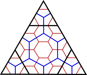
Figure 2. Three resolutions of an aperture 3 hexagon grid on a triangular face of a base polyhedron (e.g. one triangular face of an icosahedron). Notice that the orientation of the hexagons alternates at each resolution. Adapted from Sahr et al. (2003).
The Inverse Snyder Equal-Area Projection is used to project the grid onto the Earth’s surface, which is a general method projecting a platonic solid onto a sphere such that the projected polygons are equal-area while the angles and distances are slightly distorted (Snyder (1992) cited in Mocnik (2019)). The algorithm appears to be quite involved, and so I will need to rely upon existing software to implement it and create the ISEA3H grid itself.
One aspect that is often important for modelling is a method for rapidly identifying the neighbourhoods of a given cell (e.g., if modelling dispersal). Grid cells in a DGGS can be indexed in a number of ways, e.g. cells can be identified hierarchically with respect to their ‘parent’ cells at each previous resolution. While hierarchical techniques seem to be the most popular because they allow for efficient storage and retrieval, axes-based techniques are the most efficient for finding cell neighbourhoods (Mahdavi-Amiri, Samavati and Peterson, 2015). However, one difficulty is finding cell neighbourhoods that cross an edge of the underlying icosahedron.
Default indexing options in DGGRID software
By default, indexing of the grid in dggridR is by a sequence of integers 1 to the maximum number of cells. However, it is possible to obtain the ‘Q2DI’ indexing scheme. I couldn’t find documentation for the scheme, but it appears to be a triplet identifying the cell’s: (1) ‘diamond’ from the icosahedron net, and (2,3) position within the diamond resulting from the two natural axes centred on the leftmost pentagon of the diamond (e.g., Fig. 3). This indexing scheme seems similar to the Mahdavi-Amiri, Harrison and Samavati (2015) scheme (below).
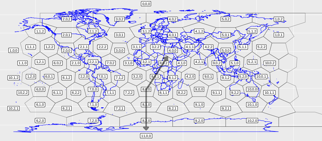
Figure 3. The resolution 2 ISEA3H with the Q2DI indexing scheme that comes built into dggridR. The opaque arrows represent the natural axes of diamond 8 in the scheme, so that each cell is indexed as: diamond number, up axis, down axis.
The Mahdavi-Amiri, Harrison and Samavati (2015) scheme
Axes-based indexing schemes are the most convenient for identifying cell neighbourhoods. Mahdavi-Amiri et al. (2015) devised an indexing scheme similar to the Q2DI above, which involves dividing the icosahedron into 10 diamonds made of up-down pairs of triangle faces, and then defining the position of each hexagonal cell within the diamond with respect to the natural axes centred on the leftmost cell (Fig. 4).
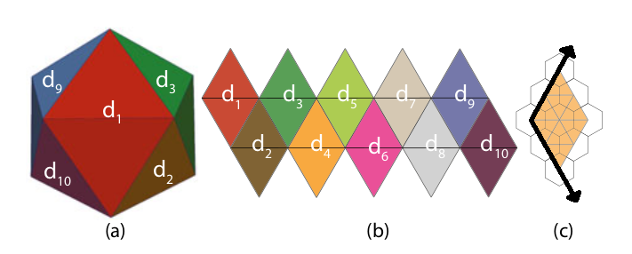
Figure 4. An icosahedron (a), the icosahedron net divided into diamond faces (b), and a resolution 2 (Class I) hexagon partitioning with the axes superimposed (c). Adapted from Mahdavi-Amiri et al. (2015).
The neighbourhood of a cell within a diamond is easily found in the Mahdavi-Amiri et al. (2015) scheme, and their Figure 14 and Table 5 provide rules for neighbourhoods that cross a diamond edge (though I believe I might have found two errors in their Table 5; see Fig. 5).
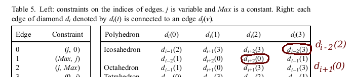
Figure 5. Possible errors in Table 5.
I partially implemented code to translate the Q2DI indices into Mahdavi-Amiri et al. (2015) indices and find cell neighbourhoods for even-resolution (Class I) grids. The code was a bit cumbersome and required a lot of case checking. For example, the pentagons at the north and south poles of the grid are their own special case. So I decided to check the literature for other ideas.
Vince (2006) scheme
Vince (2006) described an elegant scheme for indexing octahedral aperture 3 hexagonal grid (OA3H). The octahedron has the convenient property that its 6 vertices can be aligned with the three axes of the 3-dimensional Cartesian space. Then the barycentres of cells at resolution \(r\) can be given by two equations in Proposition 1, depending upon whether the resolution number is even (Class I orientation) or odd (Class II orientation, Fig. 2), which can be simplified as a triple of integers called the A3-coordinates \((a,b,c)\).
Proposition 3 in Vince (2006) gives the method of calculating the set of 6 neighbours for every cell, with a sign-changing rule if the neighbouring cell is on a different octahedral face. I think I found a missing rule for the Class II case, so I will rewrite the explanation of the proposition with my correction below.
The six neighbours of a hexagonal cell \((a,b,c)\) can be listed:
- If \(r\) is even:
- \((a+1, b-1, c)\).
- \((a-1, b+1, c)\).
- \((a+1, b, c-1)\).
- \((a-1, b, c+1)\).
- \((a, b+1, c-1)\).
- \((a, b-1, c-1)\).
- If \(r\) is odd:
- \((a+2, b-1, c-1)\).
- \((a-2, b+1, c+1)\).
- \((a-1, b+2, c-1)\).
- \((a+1, b-2, c+1)\).
- \((a-1, b-1, c+2)\).
- \((a+1, b+1, c-2)\).
The \(\pm\)’s in the above formula are to be understood subject to the following conventions. If the number \(a, b,\) or \(c\) is negative, then the sign of the operation changes. If something is subtracted from 0, then the signs of the other operations change. If \(r\) is odd and a subtraction from a positive number results in a negative, then none of the operations are performed except the sign-changing one.
Using three axes coordinates seems inefficient compared to the Mahdavi-Amiri et al. (2015) scheme above, however the rules for edge-crossing neighbourhoods are simpler, and there are no special-case cells (e.g. the north and south pole pentagons).
An indexing scheme for ISEA3H based on Vince (2006)
Indexing the vertices of the icosahedron
Vince (2006) states that, although they only applied their indexing method for the octahedron, the same method can be applied to other triangular-faced polyhedra including the icosahedron.
When the base polyhedron is an octahedron, because the 6 vertices of the octahedron can be mapped to each of the 6 positive and negative axes of a 3-dimensional Cartesian space, then an edge crossing involves a simple flip of the sign of one of the axes. The icosahedron has 6 natural axes, suggesting a 6-dimensional space, so the first thing I tried was to interpret the indices in relation to 6D Cartesian coordinates. I was able to find a way to project a 6-dimensional hypercube into 3-dimensional space to produce an icosahedron; however, I wasn’t able to find a simple indexing scheme that took advantage of this projection.
The second thing I tried was to treat each vertex of the icosahedron as an axes in a scheme similar to Vince (2006). The triangular faces of the icosahedron are analogous to the triangular faces of the octahedron in each Cartesian quadrant, so this would preserve the Vince (2006) for neighbourhoods within the face.
The question then is how to index the 12 vertices, and in a way that makes the calculation of the new face after an edge crossing as simple as possible. There are 30 edges of an icosahedron, so it would not be expensive to simply list every pair of faces corresponding to each edge crossing. However, I wondered if there was a tidy way in which the edge crossings could be calculated.
Based on the gut feeling that vertex indexing scheme should be as ‘regular’ as possible, I chose the indexing scheme in Fig. 6. It is the Hamiltonian (circuit of the icosahedron’s graph) that gives the highest degree of symmetry. As a consequence, the adjacency graph has a regular pattern, with only two ‘types’ of vertex – odd and even corresponding to inner and outer vertices in the figure – such that adjacency follows the same pattern within each type.
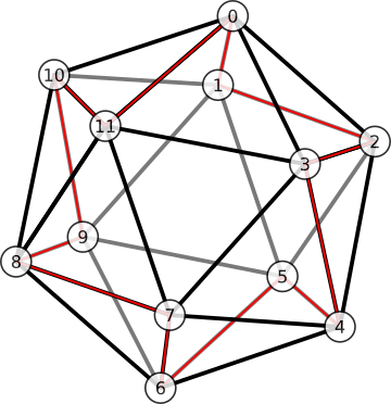
Figure 6. An indexing of vertices that produces good properties (see text). Opposite poles are always 6 apart in mod 12. The vertices can be split into two alternating types, ‘outer’ or ‘inner’, with indices that are even or odd, respectively. Then the 5 vertices adjacent to a focal vertex are always the same distances from the focal vertex (in mod 12), depending only on whether the focal vertex is odd or even.
When I use indexing scheme in Fig. 6, the opposite pole of a vertex \(v\) is simply
\[P(v) = (v + 6) \text{ mod } 12.\]For example, the opposite pole of \(v=10\) is
\[P(v=10) = (10+6) \text{ mod } 12 = 16 \text{ mod } 12 = 4.\]The indexing scheme in Fig. 6 also permits us to define vertex adjacency in a tidy way. The vertices adjacent to \(v\) can be put into an ordered list
\[\mathbf{n}_v = (v + \mathbf{s}_v) \text{ mod } 12,\]where the subscript \(v\) in \(\mathbf{s}_v\) is understood to be in mod 2, and where \(\mathbf{s}_0\) and \(\mathbf{s}_1\) are the ordered lists of distances away from vertex \(v\)
\[\begin{align} \mathbf{s}_{0} &= [10, 1, 2, 3, 11], \\ \mathbf{s}_{1} &= [1, 4, 8, 9, 11]. \end{align}\]The ordering represents clockwise circuit around \(v\) in Fig. 6. For example, the vertices adjacent to vertex 3 are
\[\begin{align} \mathbf{n}_3 &= [3+1, 3+4, 3+8, 3+9, 3+11] \text{ mod } 12, \nonumber \\ &= [4, 7, 11, 12, 13] \text{ mod } 12, \nonumber \\ &= [4, 7, 11, 0, 2]. \nonumber \end{align}\]As another example, the vertices adjacent to vertex 10 are
\[\begin{align} \mathbf{n}_{10} &= [10+10, 10+1, 10+2, 10+3, 10+11] \text{ mod } 12, \nonumber \\ &= [8, 11, 0, 1, 9]. \nonumber \end{align}\]We can also label an adjacent vertex in terms of its index in \(\mathbf{n}_v\). In the example above where vertex \(v=3\) is the focal vertex, its adjacent vertex 4 has index \(I_3(4) = 0\), so we say \(\mathbf{n}_3(0) = 4\).
For brevity below, the indices are understood to be in mod 5, i.e. \(\mathbf{n}_v(i) \rightarrow \mathbf{n}_v(i \text{ mod } 5)\), and the input into the index function is understood to be in mod 12, i.e. i.e. \(I_v(x) \rightarrow I_v(x \text{ mod } 12)\).
Two ways to cross an edge
An edge crossing is a movement from one face of the icosahedron over an edge to an adjacent face (e.g. Fig. 7). Define a face \(F\) by the triple of vertices \(F=\lbrace x, y, z \rbrace\). An adjacent face \(F' = \lbrace x', y, z \rbrace\) shares one edge with the original face \(E = \lbrace y,z \rbrace\), and it has a new vertex \(x'\) replacing \(x\).
I’ll call \(x'\) the opposite vertex of \(x\) with respect to edge \(E=\lbrace y,z \rbrace\). So we want a function
\[\omega(x, \lbrace y, z \rbrace ) = x'\]Method 1
One way we can identify the pair \(x\) and \(x'\) from the edge \(E = \lbrace y,z \rbrace\) by taking advantage of the ordering scheme above: we know that \(x\) and \(x'\) are one step away from \(z\) in \(\mathbf{n}_y\). First we identify the index corresponding to \(z\) in \(\mathbf{n}_y\), \(I_y(z)\), then the opposite vertex pair can be found
\[\begin{align} x & = n_y(I_y(z) + 1), \nonumber \\ x' & = n_y(I_y(z) - 1). \end{align}\]So one way to define \(\omega\) is
\[\begin{equation} \omega(x, \lbrace y, z \rbrace ) = n_y(I_y(z) \pm 1), \label{easier_omega} \end{equation}\]where we choose the returned value that is not \(x\).
For example, consider the edge \(E = \lbrace 7, 11 \rbrace\) in Fig. 7. Let \(y=7\) and \(z=11\), then \(\mathbf{n}_y = \mathbf{n}_7 = [8, 11, 3, 4, 6]\), and \(I_y(z) = I_7(11) = 1\). Therefore \(x = n_y(I_y(z)+1) = n_7(2) = 3\) and \(x' = n_y(I_y(z)-1) = n_7(0) = 8\).
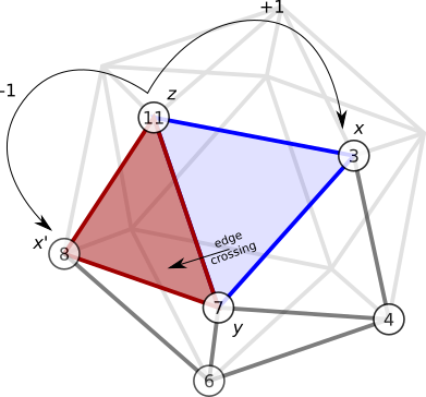
Figure 7. An example of method 1.
Method 2
Another way to find \(x'\) is to observe that it is the opposite pole of the vertex \(w\), where \(w\) is 2 ‘steps away’ from a vertex of the shared edge (Fig. 8). To formalise what is meant by 2 ‘steps away’, I can take advantage of the fact that \(\mathbf{n}_x\) describes a clockwise circuit around the vertex \(x\). The clockwise ordering scheme therefore permits us to identify a direction and a ‘maximal’ vertex of an edge pair with respect to a central vertex. In the example above, where vertex 3 is the central vertex, then the edge \(E = \lbrace 11,0 \rbrace\) has maximal element \(\text{max}( \lbrace 11, 0 \rbrace_3) = 0\). Similarly, \(\text{max}(\lbrace 9, 8 \rbrace_{10}) = 8\). We can therefore define the maximal index of an edge \(\hat{I}_v(E) = I(\text{max}(E_v))\). Then the new vertex \(x'\) can be found
\[\omega(x,E) = P(w), \text{ where } w = \mathbf{n}_x \left( \hat{I}_x(E) + 2 \right). \label{harder_omega}\]For example, consider the edge-crossing shown in Fig. 8. The original face is the face in blue, \(F = \lbrace 3, 7, 11 \rbrace\). The edge crossed is \(E = \lbrace 7, 11 \rbrace\). The vertex 11 is maximal in the clockwise direction, and counting 2 steps away from vertex 11 gives \(w = 2\). The opposite pole of \(w=2\) is \(x' = 8\). Therefore the adjacent face is \(F' = \lbrace 8, 7, 11 \rbrace\).
Figure 8. An example of method 2.
Cell neighbourhood rules
The cell index can be encoded as a list of up to 6 digits, where the first one to three digits identify the face on the icosahedron where the cell resides, and the last three digits identify its axis location according the scheme of Vince (2006)
\[c = [ v_i, v_j, v_k, h_i, h_j, h_k ],\]where the maximum \(h\) index value
\[\hat{h} = 3^{ \lfloor \frac{r+1}{2} \rfloor }.\]If the cell is on a vertex of the icosahedron, then it is one of the 12 pentagon cells. Only 1 digit of the vertex is needed to identify it, i.e.
\[c = [ v_i, -, -, \hat{h}, 0, 0 ] \text{ is a pentagon}.\]If the cell is on an edge of the icosahedron, then the two icosahedron vertices of that edge are needed, i.e.
\[c = [ v_i, v_j, -, h_i, h_j, 0 ] \text{ is a hexagonal cell on an icosahedron edge}.\]For cells in the interior of the face, all three icosahedron vertices are needed. If the vertices defining the icosahedral edge or face are always in ascending order, then each cell has a unique index.
For a focal hexagonal cell \(c = (v_i, v_j, v_k, h_i, h_j, h_k)\), the neighbouring cells \(c' = (v_i', v_j', v_k', h_i', h_j', h_k')\) can be found with similar rules to before:
- if \(r\) is even:
- \((h_i+1, h_j-1, h_k)\).
- \((h_i-1, h_j+1, h_k)\).
- \((h_i+1, h_j, h_k-1)\).
- \((h_i-1, h_j, h_k+1)\).
- \((h_i, h_j+1, h_k-1)\).
- \((h_i, h_j-1, h_k-1)\).
- if \(r\) is odd:
- \((h_i+2, h_j-1, h_k-1)\).
- \((h_i-2, h_j+1, h_k+1)\).
- \((h_i-1, h_j+2, h_k-1)\).
- \((h_i+1, h_j-2, h_k+1)\).
- \((h_i-1, h_j-1, h_k+2)\).
- \((h_i+1, h_j+1, h_k-2)\).
The additional rules are needed to handle edge-crossing:
- If something is subtracted from \(h_k = 0\) so \(h'_k < 0\), then:
- \(v_k' = \omega(v_k, (v_i,v_j) )\).
- the sign of \(h'_k\) is swapped;
- the signs of the other operations are swapped and \(h_i'\) and \(h_j'\) recalculated
- If something is subtracted from \(h_k \neq 0\) so \(h'_k < 0\), then:
- \(v_k' = \omega(v_k, (v_i,v_j) )\).
- the new hexagon indices are the same as the old, i.e. \((h_i', h_j', h_k') = (h_i, h_j, h_k)\)
For a focal pentagonal cell \(c = (v_i, -, -, \hat{h}, 0, 0)\),
- if \(r\) is even then \(c' = (v_i, \mathbf{n}_{v_i}(x), -, \hat{h}-1, 1, 0)\) for \(x = 0, \ldots, 4\).
- else if \(r\) is odd then \(c' = (v_i, \mathbf{n}_{v_i}(x), \mathbf{n}_{v_i}(x+1), \hat{h}-2, 1, 1)\) for \(x = 0, \ldots, 4\).
Implementation
I’ve put some code on Github. In order to run it, you’ll need both rgdal and dggridR. The dggridR package has since been removed from CRAN, so you will need to install from the archive.
First, install the prerequisite packages, on the commandline:
$ sudo apt-get install r-cran-rgdal
$ sudo apt-get install r-cran-devtools
To install dggridR from the archive, in R:
> library('devtools')
Loading required package: usethis
> install_url('https://cran.r-project.org/src/contrib/Archive/dggridR/dggridR_2.0.4.tar.gz')
# Chose Update All when prompted
Then to run the code I put on Github, in R:
> library(dplyr)
> library(dggridR)
> source("Q2DI_to_V.R")
> source("get_V_label.R")
> source('find_neighbours_V.R')
> source('plot_vince_wneighs.R')
> plot_vince(3) # 3 refers to a resolution 3 grid
This should produce a pdf that looks like Fig. 9.
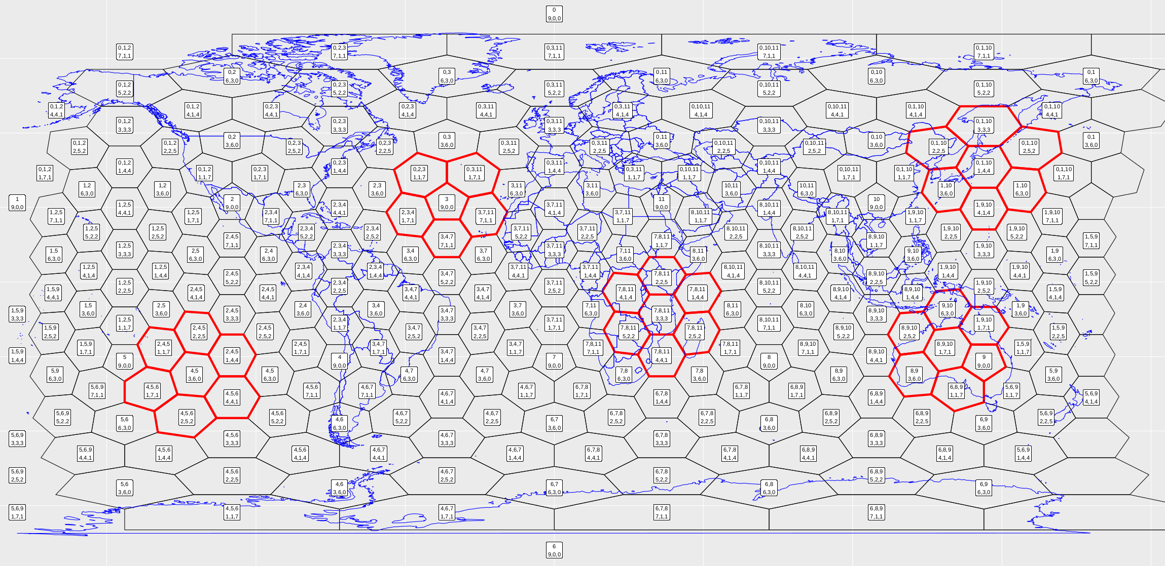
Figure 9. Running the snippet of code above should produce this figure. Each cell is labelled according to the new indexing scheme. I’ve also chosen five cells and found their neighbourhoods, highlighted in red.
To run it for different resolution, just change the variable:
> plot_vince(4) # 4 refers to a resolution 4 grid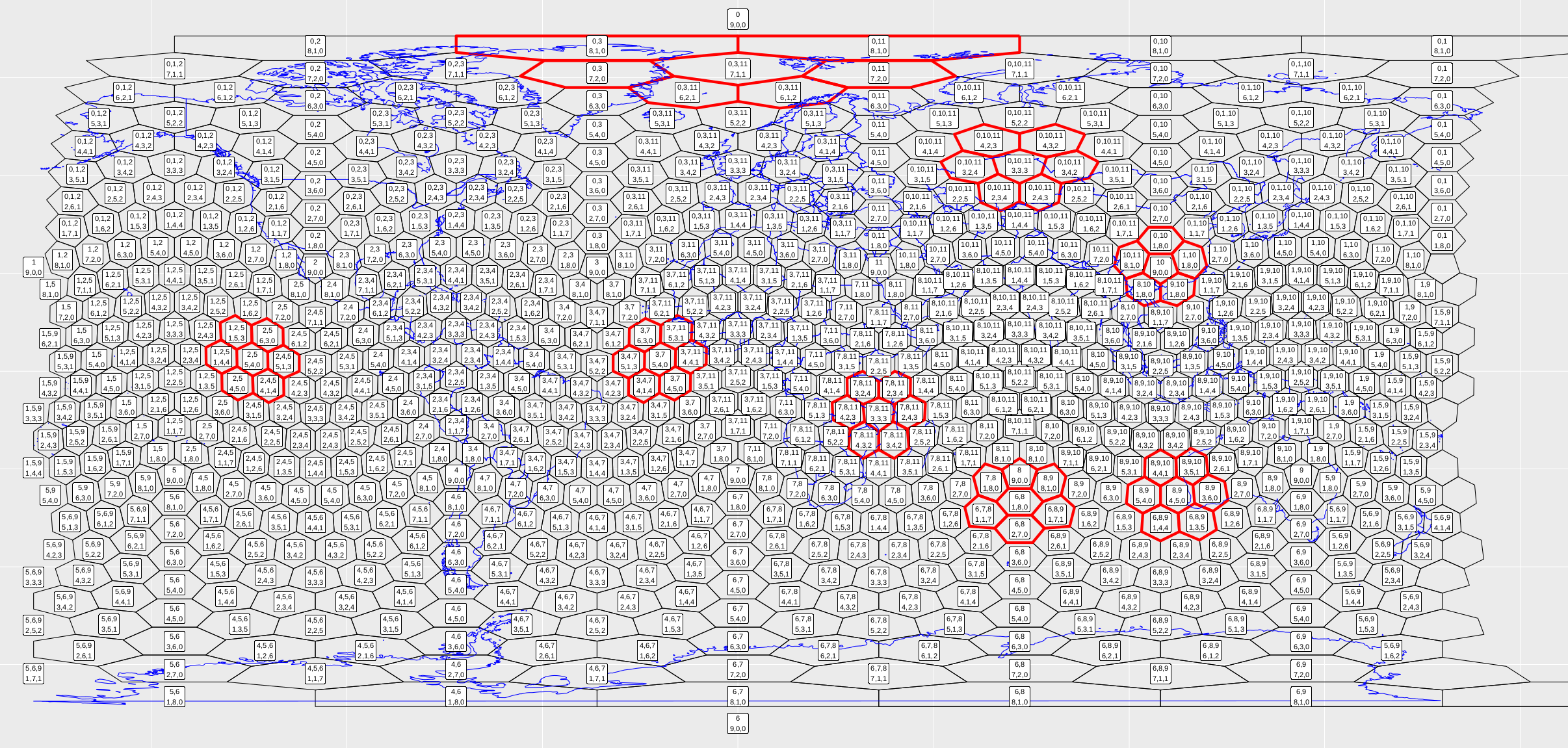
Figure 10. Running the snippet of code above should produce this figure.
The code is no way optimised (more a proof of concept), so resolution 4 is about as far as I would go.
References
Barnes, R. (2017). dggridR: Discrete Global Grids for R. R package version 0.1.12. URL: https://github.com/r-barnes/dggridR/
Mahdavi-Amiri, A., Harrison, E. and Samavati, F. (2015). Hexagonal connectivity maps for digital earth, International Journal of Digital Earth 8(9): 750–769.
Mahdavi-Amiri, A., Samavati, F. and Peterson, P. (2015). Categorization and conversions for indexing methods of discrete global grid systems, ISPRS International Journal of GeoInformation 4(1): 320–336.
Mocnik, F.-B. (2019). A novel identifier scheme for the isea aperture 3 hexagon discrete global grid system, Cartography and Geographic Information Science 46(3): 277–291.
Sahr, K. (2018). DGGRID version 6.4: User documentation for discrete global grid software, Southern Terra Cognita Laboratory. URL: https://discreteglobalgrids.org/wp-content/uploads/2019/05/dggridManualV64.pdf
Sahr, K., White, D. and Kimerling, A. J. (2003). Geodesic discrete global grid systems, Cartography and Geographic Information Science 30(2): 121–134.
Vince, A. (2006). Indexing the aperture 3 hexagonal discrete global grid, Journal of Visual Communication and Image Representation 17(6): 1227–1236.