Link distribution in static community models like the niche model
I was recently reading a 2006 review of food web structure by Jennifer Dunne, which includes a very thorough discussion of static community models like the niche model (Williams & Martinez 2000, Nature), and I was struck again by how unclear it is - to me, anyway - what exactly it is that these static models represent.
There’s no doubt that they do an excellent job of replicating the coarse structural properties of large empirical food webs. They also provide important concrete evidence that food web structure is non-random, and a set of simple rules that replicate this structure … simple rules which offer tantalising hints about mechanisms underlying that structure. But even in discussing the intervality property, which has been in the literature for quite a while, Dunne (2006, Ecological Networks: Linking Structure to Dynamics in Food Webs) observes that why species should be able to be represented by a single dimension, or what the single dimension might represent, “continues to be unclear”. The clearest hypothesis has been about the role of body size, which some workers have taken and run with (e.g. the Louielle & Loreau (2005, PNAS) model), but is obviously restricted in its applicability.
It has been a while since I’ve read this literature, so I’ve been reading forward to see what the latest developments have been. One key paper I found was Stouffer et al. (2005, Ecology), who identifies two key properties underlying the success of the niche and nested-hierarchy models:
- The niche values to which species are assigned form a totally ordered set.
- Each species has a specific probability x of preying on species with lower niche values, where x is drawn from an approximately exponential distribution.
The first condition looks like a kind of weakening of the original intervality property, which might (or might not) be related to body size. The second condition however, what does that mean?
I started by taking a peek back at the code I wrote up to create webs using the niche model. The important lines are:
ni = rand; % the random niche value
y = rand;
ri = ni*(1-(1-y)^(1/beta)); % or ri = ni*x
ci = rand*(ni-ri/2)+ri/2;
That ri value is the range of niche values over which a particular species can predate. The bigger that is, the more prey a species has. The x to which Stouffer et al. (2005, Ecology) refers is the second half of the product that forms ri, the (1-(1-y)^(1/beta)) term.
What do those x values look like?
I generated a bunch of them using portions of the code above and plotted a histogram of them below. The y-axis is the frequency and the x-axis is the value of Stouffer’s x.
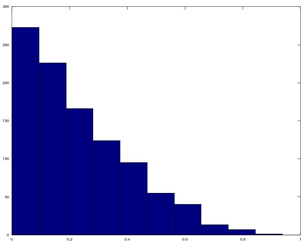
Frequency histogram of x values, which determine the size of the range of niche values upon which a predator can feed.
As Stouffer puts it, the x values are drawn from an approximately exponential distribution. In other words, many predators have few prey, and a few predators have many prey.
So what does this do to the shape of the web?
Stouffer shows that if the original cascade model is modified to satisfy condition 2 above, then it performs about as well as the niche model. Originally, the Cascade model had it so a species with a lower niche value than another species becomes its prey with a fixed probability of 2CS/(S-1). So one way to assign prey would be like this:
cascade_x = 2*C*S/(S-1);
cascade_no_prey = zeros(S,1);
for i = 1:S
    potl_prey = find(n<n(i));
    for j = 1:length(potl_prey)
        if rand > cascade_x
            cascade_no_prey(i) += 1;
        end
    end
end
In the generalised cascade model - the one Stouffer et al. created to satisfy condition 2 - prey would be assigned like in the niche model:
gen_cascade_no_prey = zeros(S,1);
for i = 1:S
    potl_prey = find(n<n(i));
    predator_specific_x = (1-(1-rand).^(1/beta));
    for j = 1:length(potl_prey)
        if rand > predator_specific_x
            gen_cascade_no_prey(i) += 1;
        end
    end
end
Using the Little Rock Lake S (number of species) and C parameters, I plotted the niche value of each species below (x-axis) against the number of prey it has (y-axis). The cascade model (in blue) describes a fairly linear relationship between a species’ niche value and the number of prey it has. The higher a species in the web, the more species it predates upon. In contrast, the generalised cascade model (in red) has a much more spread-out relationship - mostly spread downwards. So while it’s still generally true that species higher in the web have a larger number of prey, it’s not always true, and some species high in the web have very few prey.

Choosing x values from the approximately exponential distribution results in a model in which some top predators have few prey, compared to the original cascade model
If I had to guess, I’d say that this contrast between the two models, the relative success of the condition-2-satisfying models, says something about specialisation. The straight body-size hypothesis implies that a predator can eat anything that is smaller than it, and so the higher the body size (i.e. the higher the niche value), the larger the range of potential prey. But predator-prey relationships are an arms-race, predators are forced to specialise, and so some predators will have a restricted range of prey.
… Though I suppose “specialisation” in this case is another way of saying “additional niche dimensions”, which goes to the heart of why there’s a niche hierarchy, its historical roots in intervality, in the first place.
Additional bits:
- My code for the second figure: distributions.m
- Bookmark to read later: Stouffer, 2010 Functional Ecology.