Cooperation among unequals
In an unpublished paper, Staab et al. (2022) studied the effects of heterogeneity in endowments and productivities on cooperation. They were particularly interested in the effect of allowing players to share the jointly produced goods unequally. Surprisingly, they found that unequal sharing can promote cooperation.
In this blog post, first, I offer a proof of one of their propositions. Then I try thinking about their model a little differently to how they presented it, working through some small examples to try to get a visual intuition for what it means.
Signs of eigenvalues proof
Staab et al. (2022) model an \(n\)-player iterated public goods game with a continuation probability \(\delta\). Each round, individual \(i\) receives endowment \(e_i\) that they can either contribute to the public good or keep. Their strategy is deterministic and fixed for all rounds. If individual \(i\) contributes to the public good, their contribution is multiplied by their productivity \(r_i\). The return from the public good is shared among the members of the group according to a sharing rule \(\boldsymbol{f} = (f_1, \ldots, f_n)\), where \(f_i\) is the proportion of the jointly produced good that individual \(i\) receives.
The optimal sharing rule and minimum continuation probability pair \((\boldsymbol{f}^*, \delta_{\text{min}})\) solves an eigenvalue problem
\[\begin{equation*} \delta_{\text{min}} \boldsymbol{f}^* = \Phi \boldsymbol{f}^*, \end{equation*}\]where the matrix \(\Phi\) has elements
\[\begin{equation} \phi_{ij} = \begin{cases} \frac{-e_i (r_i - 1)}{\sum_{k \neq i} e_k r_k}, & i = j, \\ \frac{e_i}{\sum_{k \neq i} e_k r_k}, & i \neq j. \end{cases} \label{phi_ij} \tag{1} \end{equation}\]In Proposition 4, they state:
“the optimal sharing rule [\(f^*\)] is the eigenvector that corresponds to the largest eigenvalue of the matrix \(\Phi\)”
and
“the largest eigenvalue is the minimal continuation probability (\(\delta_{\text{min}})\) for this sharing rule to be feasible”
Below, I offer a proof that \(\delta_{\text{min}}\) is indeed the largest eigenvalue — the only eigenvalue that has the potential to be positive — and that it is positive only when their Assumption 1 is satisfied (non-triviality of cooperation):
\[\begin{equation} \sum_i \frac{1}{r_i} > 1. \label{reciprocal_productivity_condition} \tag{2} \end{equation}\]The theorem can be proved by analysing the characteristic polynomial of \(\Phi\) using a similar approach to Meyer (2000, Ex. 7.1.22).
Let \(\Phi\) be the matrix defined by Eq. \ref{phi_ij}. Then:
- At least \(n-1\) eigenvalues of \(\Phi\) are negative.
- The largest eigenvalue \(\lambda_1\) of \(\Phi\) is positive if and only if the reciprocal productivity condition from Assumption 1 (Eq. \ref{reciprocal_productivity_condition}) is satisfied.
Proof. Matrix \(\Phi\) can be rewritten as a rank-one update of a diagonal matrix (e.g., Meyer, 2000, Sect. 6.2)
\[\begin{equation*} \Phi = D + \boldsymbol{b} \boldsymbol{1}^T, \end{equation*}\]where \(D\) is a diagonal matrix with elements
\[\begin{equation*} d_i = \frac{- e_i r_i}{\sum_{k \neq i} e_k r_k} < 0, \end{equation*}\]and \(\boldsymbol{b}\) is a column vector with elements
\[\begin{equation*} b_i = \frac{e_i}{\sum_{k \neq i} e_k r_k} > 0. \end{equation*}\]Consider the corresponding eigenvalue problem
\[\begin{equation*} \lambda \boldsymbol{v} = (D + \boldsymbol{b} \boldsymbol{1}^T) \boldsymbol{v} = D \boldsymbol{v} + \boldsymbol{b} \boldsymbol{1}^T \boldsymbol{v} = D \boldsymbol{v} + c \boldsymbol{b}, \end{equation*}\]where \(\boldsymbol{1}^T \boldsymbol{v} = c\) is a constant. Rearrange to obtain \(1 = \boldsymbol{1}^T (\lambda I - D)^{-1} \boldsymbol{b}\). Since \(\lambda I - D\) is a diagonal matrix, \((\lambda I - D)^{-1}\) is also a diagonal matrix but with reciprocal elements to the original. Therefore, the eigenvalues solve \(1 = \sum_{i=1}^n \frac{b_i}{\lambda - d_i}\), which can be rearranged to obtain the characteristic polynomial of \(\Phi\):
\[\begin{equation*} f(\lambda) = \prod_{i=1}^n (\lambda - d_i) - \sum_{i=1}^n b_i \prod_{j\neq i} (\lambda - d_j). \end{equation*}\]To partition the repeated and unique eigenvalues, we factorise the characteristic polynomial \(f(\lambda)\). First, we index the unique diagonal elements of \(D\) in descending order \(d_{(1)} > d_{(2)} > ... > d_{(m)}\), where \(m \leq n\), and define the corresponding index sets:
\[\begin{equation*} I_{(i)} \equiv \left\{j \in \{1, 2, \ldots, n\} \mid d_j = d_{(i)}\right\}. \end{equation*}\]Second, we define the sum of \(b_j\) elements in the same index set:
\[\begin{equation*} B_{(i)} \equiv \sum_{j \in I_{(i)}} b_j. \end{equation*}\]Then we can factorise the characterisic polynomial as \(f(\lambda) = g(\lambda) h(\lambda)\), where
\[\begin{equation*} g(\lambda) = \prod_{l=1}^m (\lambda - d_{(l)})^{|I_{(l)}|-1} , \end{equation*}\]and
\[\begin{equation} h(\lambda) = \prod_{k=1}^m (\lambda - d_{(k)}) - \sum_{i=1}^m B_{(i)} \prod_{j \neq i} (\lambda - d_{(j)}). \label{h(lambda)} \tag{3} \end{equation}\]Example 1. Consider a game played with \(\boldsymbol{e} = (0.2, 0.2, 0.2, 0.4)\) and \(\boldsymbol{r} = (2, 2, 2, 3)\). Then
\[\begin{align*} \Phi & = \begin{pmatrix} -0.10 & 0.10 & 0.10 & 0.10 \\ 0.10 & -0.10 & 0.10 & 0.10 \\ 0.10 & 0.10 & -0.10 & 0.10 \\ 0.33 & 0.33 & 0.33 & -0.67 \\ \end{pmatrix} \\ &= \underbrace{ \begin{pmatrix} -0.2 & 0 & 0 & 0 \\ 0 & -0.2 & 0 & 0 \\ 0 & 0 & -0.2 & 0 \\ 0 & 0 & 0 & -1.0 \\ \end{pmatrix} }_{D} + \underbrace{ \begin{pmatrix} 0.10 & 0.10 & 0.10 & 0.10 \\ 0.10 & 0.10 & 0.10 & 0.10 \\ 0.10 & 0.10 & 0.10 & 0.10 \\ 0.33 & 0.33 & 0.33 & 0.33 \\ \end{pmatrix} }_{\boldsymbol{b} \boldsymbol{1}^T} \end{align*}\]The characteristic polynomial
\[\begin{equation*} f(\lambda) = (\lambda + 0.2)^3 (\lambda+1) - 0.3 (\lambda + 0.2)^2 (\lambda + 1) - 0.33(\lambda + 0.2)^3. \end{equation*}\]Indexing the unique diagonal elements:
\[\begin{alignat*}{6} &d_{(1)} &&= -0.2, \qquad &&I_{(1)} &&= \{ 1, 2, 3 \}, \qquad &&B_{(1)} &&= 0.3, \\ &d_{(2)} &&= -1, \qquad &&I_{(2)} &&= \{ 4 \}, \qquad &&B_{(2)} &&= 0.33. \end{alignat*}\]So the characteristic polynomial can be factorised as
\[\begin{equation*} f(\lambda) = \underbrace{ \left[ (\lambda + 0.2)^2 \right] }_{g(\lambda)} \underbrace{ \left[ (\lambda + 0.2) (\lambda + 1) - 0.3 (\lambda + 1) - 0.33 (\lambda + 0.2) \right] }_{h(\lambda)}. \end{equation*}\]The roots of \(g(\lambda)\) correspond to the repeated diagonal elements of \(D\), which are all negative. Specifically, for each unique diagonal element \(d_{(\ell)}\) with multiplicity \(|I_{(\ell)}| > 1\), \(g(\lambda)\) contributes \(|I_{(\ell)}| - 1\) roots to the characteristic polynomial \(f(\lambda)\), and these roots are equal to \(d_{(\ell)}\). The roots of \(g(\lambda)\) correspond to the eigenvalues of \(\Phi\) that are unchanged by the rank-one update. Since \(d_{(\ell)} < 0\) for all \(\ell\) (due to the definition of \(D\)), the roots of \(g(\lambda)\) correspond to negative eigenvalues of \(\Phi\). The total number of such eigenvalues is \(\sum_{\ell=1}^m (|I_{(\ell)}| - 1) = n - m\). Therefore, \(g(\lambda)\) accounts for \(n - m\) negative eigenvalues of \(\Phi\).
The remaining \(m\) eigenvalues are determined by the roots of \(h(\lambda)\). To characterise them, we will show that:
- \(h(d_{(\ell)})\) alternates in sign with \(\ell\) according to: \(\text{sign}(h(d_{(\ell)})) = (-1)^\ell\) for \(\ell = 1, \ldots, m\).
- \(h(L) > 0\) for sufficiently large \(L\).
- \(h(0) < 0\) if and only if \(\sum_{i=1}^n \frac{1}{r_i} > 1\) (the reciprocal productivity condition).
To show Point 1, we analyse the signs of the terms in Eq. \ref{h(lambda)}. First, we can simplify \(h(d_{(\ell)})\)
\[\begin{align*} h(d_{(\ell)}) &= \underbrace{\prod_{k=1}^m (d_{(\ell)} - d_{(k)})}_{0} - \sum_{i=1}^m B_{(i)} \underbrace{\prod_{j \neq \ell} (d_{(\ell)} - d_{(j)})}_{0 \text{ except when } i = \ell}, \\ &= -B_{(\ell)} \prod_{j \neq \ell} (d_{(\ell)} - d_{(j)}). \end{align*}\]From the ordering \(d_{(1)} > d_{(2)} > ... > d_{(m)}\), the signs of the terms in the product are known:
\[\begin{equation*} \text{sign}(d_{(\ell)} - d_{(j)}) = \begin{cases} +1 & \text{ if } \ell < j, \\ -1 & \text{ if } \ell > j. \end{cases} \end{equation*}\]Therefore, \(h(d_{(\ell)})\) is the product of: the negative term \(-B_{(\ell)}\), \(\ell-1\) negative terms, and \(m - \ell\) positive terms. Consequently, \(\text{sign}(h(d_{(\ell)})) = (-1)^{\ell}\).
Example 2. Show that \(h(d_{(1)}) < 0\) and \(h(d_{(2)}) > 0\).
For \(h(d_{(1)})\):
\[\begin{align*} h(d_{(1)}) &= \underbrace{\prod_{k=1}^m (d_{(1)} - d_{(k)})}_{0} - \sum_{i=1}^m B_i \underbrace{\prod_{j \neq i} (d_{(1)} - d_{(j)})}_{0 \text{ except when } i = 1}, \\ &= - B_{(1)} \prod_{j \neq 1} \underbrace{(d_{(1)} - d_{(j)})}_{d_{(1)} > d_{(j)} \forall j \neq 1} < 0. \end{align*}\]For \(h(d_{(2)})\):
\[\begin{align*} h(d_{(2)}) &= \underbrace{\prod_{k=1}^m (d_{(2)} - d_{(k)})}_{0} - \sum_{i=1}^m B_i \underbrace{\prod_{j \neq i} (d_{(2)} - d_{(j)})}_{0 \text{ except when } i = 2}, \\ &= - B_{(2)} \prod_{j \neq 2} (d_{(2)} - d_{(j)}), \\ &= - B_{(2)} \underbrace{(d_{(2)} - d_{(1)})}_{(-)} \underbrace{(d_{(2)} - d_{(3)})}_{(+)} \underbrace{(d_{(2)} - d_{(4)})}_{(+)} \ldots \underbrace{(d_{(2)} - d_{(m)})}_{(+)} \\ &> 0. \end{align*}\]To show Point 2, we show that there exists some large-enough \(L\) such that \(h(L) > 0\). Rearranging Eq. \ref{h(lambda)}:
\[\begin{equation*} h(L) = \underbrace{\left( \prod_{k=1}^m \left( L - d_{(k)} \right) \right)}_{\text{LHT}} \underbrace{\left( 1 - \sum_{i=1}^m \frac{B_{(i)}}{L - d_{(i)}} \right)}_{\text{RHT}}. \end{equation*}\]If \(L > d_{(1)}\), then the left-hand term \(\text{LHT} > 0\). If \(\sum_{i=1}^m \frac{B_{(i)}}{L - d_{(i)}} < 1\), then the right-hand term \(\text{RHT} > 0\). We observe:
\[\begin{equation*} \sum_{i=1}^m \frac{B_{(i)}}{L - d_{(i)}} < \sum_{i=1}^m \frac{\text{max}(\{B_{(i)}\})}{L - d_{(i)}} < m \frac{\text{max}(\{B_{(i)}\})}{L - d_{(1)}}. \end{equation*}\]Therefore, if \(L > m \cdot \text{max}(\{B_{(i)}\}) + d_{(1)}\), then \(h(L) > 0\).
To show Point 3, we substitute \(\lambda = 0\) into Eq. \ref{h(lambda)}
\[\begin{equation*} h(0) = \left(\prod_{k=1}^m (- d_{(k)}) \right) \left( 1 - \sum_{i=1}^n \frac{1}{r_i} \right). \end{equation*}\]The left-hand term is positive. Therefore, \(h(0) < 0\) if and only if \(\sum_{i=1}^n \frac{1}{r_i} > 1\).
Using Points 1, 2, and 3 to analyse the sign of \(h(\lambda)\), we can locate the roots and identify the signs of the eigenvalues of \(\Phi\).
Example 3. Consider a 5-player game with
\[\boldsymbol{e} = (0.3, 0.2, 0.2, 0.2, 0.1)\]and
\[\boldsymbol{r} = (4, 3, 3, 3, 2)\]which gives
\[\boldsymbol{d} = (-0.60, -0.23, -0.23, -0.23, -0.07)\]The figure below shows the relationship between the characteristic polynomial \(f(\lambda)\), its factor \(h(\lambda)\), the unique diagonal elements of \(D\) \(d_{(i)}\), and the eigenvalues of \(\Phi\). The repeated eigenvalues correspond to repeated \(d_i\). Function \(h(\lambda)\) alternates in sign at each unique \(d_i\). The sign of the largest eigenvalue \(\lambda_1\) is determined by the sign of \(h(0)\).
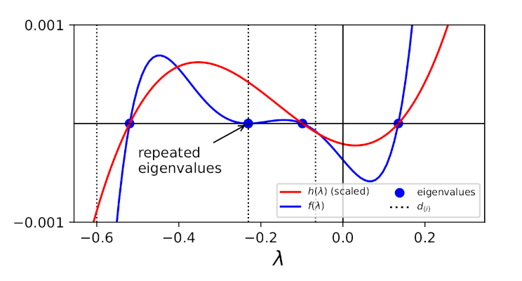
From Point 1, we know that \(h(\lambda)\) has \(m\) roots strictly interlacing the \(d_{(\ell)}\) values. The \(d_{(\ell)}\) values are negative. Therefore, \(m-1\) roots satisfy \(d_{(\ell + 1)} < \lambda < d_{(\ell)}\) and are negative.
The \(m-1\) negative roots of \(h(\lambda)\) combine with the \(n-m\) negative roots of \(g(\lambda)\) to account for \(n-1\) eigenvalues of \(\Phi\). Therefore, we can conclude that at least \(n-1\) eigenvalues of \(\Phi\) are negative.
The remaining root of \(h(\lambda)\) might satisfy either \(\lambda < d_{(m)}\) or \(\lambda > d_{(1)}\). From Point 2, since \(h(d_{(1)}) < 0\) and \(h(L) > 0\) for some large \(L\), then the remaining root must be the largest root of \(\Phi\) and satisfy \(d_{(1)} < \lambda_1 < L\). Therefore, in summary so far, we have
\[\begin{equation*} \overbrace{d_{(m)} < \lambda_m < d_{(m-1)} < \ldots < d_{(2)} < \lambda_2 < \underbrace{d_{(1)}}_{(-)}}^{\text{$m-1$ negative roots of $h(\lambda)$ interlacing $d_{(1)}$ to $d_{(m)}$}} < \lambda_1 < \underbrace{L}_{(+)}. \end{equation*}\]The sign of \(\lambda_1\) is determined by the sign of \(h(0)\). In particular, \(\lambda_1 > 0\) if and only if \(h(0) < 0\). From Point 3, \(h(0) < 0\) if and only if \(\sum_{i=1}^n 1/r_i > 1\), where the latter is the reciprocal productivity condition from Assumption 1 (Eq. \ref{reciprocal_productivity_condition}). Therefore, we conclude that \(\lambda_1 > 0\) if and only if Assumption 1 is satisfied.
Try to get a visual intuition
The folk theorem tells us that, if players in an iterated game are sufficiently patient (i.e., the discount factor \(\delta \rightarrow 1\)), then any feasible and individually rational average payoff can be sustained in a subgame-perfect equilibrium via a generalised Grim-trigger strategy. In particular, taking into account that the Nash equilibrium of the stage game NE is a subgame-perfect equilibrium, then a player will be willing to stick to any alternative strategy to NE, call it ALT, so long as the payoff from ALT is greater than or equal to the maximum payoff they could obtain from a one-shot deviation (MAX DEVN) plus reversion to NE for the remainder of the game
\[\begin{equation} \pi_k(\text{ALT}) \geq (1 - \delta) \; \pi_k(\text{MAX DEVN}) + \delta \; \pi_k(\text{NE}). \end{equation}\]The following equation is given (between Eqs. 1 and 2 in Staab et al.) for the Grim strategy
\[\begin{equation} \underbrace{f_k \sum_i e_i \; r_i}_{\text{payoff from full coop}} \geq \underbrace{(1 - \delta) \; f_k \; \sum_{j \neq k} e_j \; r_j + e_k}_{\text{payoff from one-shot devn + reversion}}. \label{eq:staab_1.5} \tag{4} \end{equation}\]We could generalise this a bit to obtain the space of feasible rational payoffs of all alternative strategies.
First, the frontier of the feasible set is defined by the payoffs from full cooperation with \(\sum_i f_i = 1\). Second, the maximum possible payoff that focal player \(k\) can obtain from a one-shot deviation occurs when: player \(k\)’s deviation is to defect instead of cooperate, and the deviation is timed to occur when all non-focal players choose cooperate. Therefore, the right-hand side of Eq. \ref{eq:staab_1.5} defines the bounds of the individually rational set. Therefore, the set of feasible and rational alternative-strategy payoffs are the values between the left- and right-hand sides of Eq. \ref{eq:staab_1.5}
\[\begin{equation} \underbrace{f_k \sum_i e_i \; r_i}_{\text{payoff from full coop}} \geq \pi_k(\text{ALT}) \geq \underbrace{(1 - \delta) \; f_k \; \sum_{j \neq k} e_j \; r_j + e_k}_{\text{payoff from one-shot devn + reversion}}. \label{eq:my_staab_1.5} \tag{5} \end{equation}\]When \(\delta = 1\), Eq. \ref{eq:my_staab_1.5} reduces to
\[\begin{equation*} \underbrace{f_k \sum_i e_i \; r_i}_{\text{payoff from full coop}} \geq \pi_k(\text{ALT}) \geq e_k, \end{equation*}\]where \(\boldsymbol{e}\) has the natural interpretation as the disagreement point.
As \(\delta\) increases, the space between the left- and right-hand sides Eq. \ref{eq:my_staab_1.5} contracts until we find the point where
\[\begin{equation*} \underbrace{f_k^* \sum_i e_i \; r_i}_{\text{payoff from full coop}} = \pi_k(\text{ALT}) = \underbrace{(1 - \delta^*) \; f_k^* \; \sum_{j \neq k} e_j \; r_j + e_k}_{\text{payoff from one-shot devn + reversion}}. \end{equation*}\]It is finding this point that is the main focus of Staab et al.; in particular, finding the value of the pair \((\boldsymbol{f}^*, \delta^*)\).
A visual example
Consider a 2-player scenario where
\[\begin{equation*} \boldsymbol{e} = (0.2, 0.8), \text{ and } \boldsymbol{r} = (2, 1.5). \end{equation*}\]At full cooperation, the maximum possible quantity of goods is produced
\[\begin{equation*} g = e_1 \; r_1 + e_2 \; r_2 \end{equation*}\]When those goods are efficiently shared, i.e., \(f_1 + f_2 = 1\), each player receives
\[\begin{align*} \pi_1 &= f_1 \; g, \\ \pi_2 &= (1 - f_1) \; g. \end{align*}\]This describes the function that defines the upper limit of the feasible set, i.e., the frontier, which is shown as a blue line in Fig. 1.
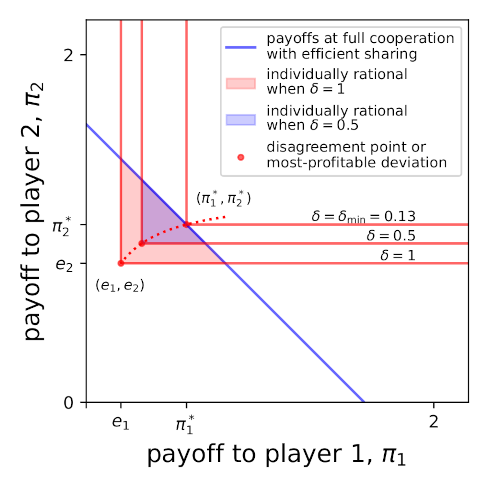
Figure 1. A two-player example.
If the game is repeated forever, i.e., the continuation probability \(\delta = 1\), then the maximum deviation payoff players can receive is equal to the payoff from private investment
\[\begin{equation*} \text{max. deviation payoff}_k = e_k. \end{equation*}\]For each player \(k\), this is the minimum game payoff that a rational player should be willing to receive from the game, which are shown by red lines in Fig. 1.
Combining the upper limit defining the feasible set and the lower limits defining the minimum individually rational payoffs for all players defines the feasible and rational payoffs region (shaded red in Fig. 1). Any combination of strategies and sharing agreements (\(\boldsymbol{f}\)) that provide payoffs within this region can be sustained.
If the continuation probability \(\delta < 1\), then the maximum deviation payoff (normalised) includes the payoff from the deviation-round itself
\[\begin{equation*} \text{max. deviation payoff}_k = e_k + (1-\delta) \; f_k \; \sum_{j \neq k} e_j r_j. \end{equation*}\]Therefore, decreasing \(\delta\) shrinks the feasible rational region (e.g., when \(\delta = 0.5\), the region shrinks to the blue shaded region in Fig. 1), which reduces the number of strategies and sharing agreements that can be sustained.
Staab et al. are interested in finding the \(\delta_{\text{min}}\) for which the feasible-rational region shrinks to a single point. In Fig. 1, this point occurs when \(\delta = \delta_{\text{min}} = 0.13\), which corresponds to payoffs \((\pi_1^*, \pi_2^*) \approx (0.58, 1.02)\) on the frontier, with sharing agreement \((f_1^*, f_2^*) \approx (0.36, 0.64)\).
Some more examples
Productivities equal, vary outside options
Consider an example with equal productivities
\[\begin{equation*} \boldsymbol{r} = (1.5, 1.5) \end{equation*}\]where we vary the outside options (Fig. 2). The poorer player receives the smaller share, e.g., for the purple line, Player 1 is the poorer player.
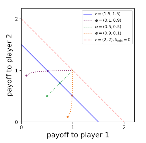
Figure 2. Two-player examples with equal productivities and different outside options. Note that the distance along the critical-point line is not reliably indicative of \(\delta_{\text{min}}\). For the unequal-endowments scenarios, \(\delta_{\text{min}} \approx 0.11\), whereas for the equal-endowments scenario, \(\delta_{\text{min}} \approx 0.33\).
We can predict the outcomes of higher and lower productivity levels — while keeping \(r_1 = r_2\) — by moving the frontier (blue line) up and down. When productivities are low, \(\delta_{\text{min}} \rightarrow 1\), and the shares reflect the outside option. But as productivity increases, \(\delta_{\text{min}}\) decreases, and the shares become more equal. The shares meet at equal shares, which occurs when \(r\) is high enough that it no longer presents a social dilemma. At this point, \(\delta_{\text{min}} = 0\), which makes this a one-shot game.
What does it mean that players demand an equal share in the one-shot game, regardless of their outside option? When \(\boldsymbol{r} = (2, 2)\), the payoffs they receive from the game are greater than their outside options. But recall that the fact a cooperative solution gives both players higher payoffs is not enough to guarantee it. From the eigenvalues proof, we need the leading eigenvalue \(\lambda_1 = 0\), which implies \(h(0) = 0\), which implies \(\sum_i 1/r_i = 1\). For equal \(r_i\), that implies \(r_i = 2\). The social dilemma condition is that the return on investment is less than one
\[\begin{equation*} f_k \; r_k < 1 \text{ for all } k \in \mathcal{N} \end{equation*}\]and, when \(r_k = 2\), this condition is only satisfied by \(f_k = 0.5\).
Or to think about it another way, when \(r_i = 2\), the situation is on the cusp of transition from PD to mutualism. The payoff matrix is
| C | D | |
|---|---|---|
| C | 1, 1 | 0.1, 1 |
| D | 1, 0.9 | 0.1, 0.9 |
where the calculation for the cooperative payoff is
\[\begin{equation*} \pi_1(C, C) = f_1 (e_1 \; r_1 + e_2 \; r_2) = 0.5 ( 0.9 \times 2 + 0.1 \times 2) = 1, \end{equation*}\]and the deviations (off-diagonal elements of the payoff matrix) are
\[\begin{equation*} \pi_1(D, C) = f_1 \; e_2 \; r_2 + e_1 = 0.5 \times 0.9 \times 2 + 0.1 = 1, \end{equation*}\]and
\[\begin{equation*} \pi_2(C, D) = f_2 \; e_1 \; r_1 + e_2, = 0.5 \times 0.1 \times 2 + 0.9 = 1. \end{equation*}\]Productivities unequal
In this final subsection, I tried playing around with an example with unequal productivities, approaching it from different angles to see if it could help my intuition.
Consider an example with unequal productivities
\[\begin{equation*} \boldsymbol{r} = (1.1, 2.2) \end{equation*}\]and use Fig. 3 as our guide. I’m curious about the point where the disagreement-point trajectory hits the diagonal line, the special points marked with stars in Fig. example_3 and the grey line they align upon.
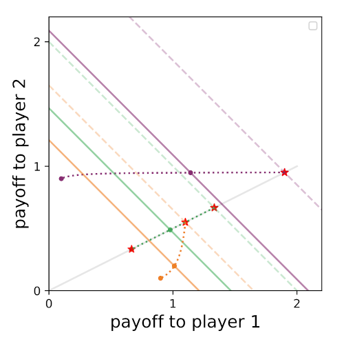
Figure 3. Two-player examples with unequal productivities. Player 2 is the more productive player.
The dashed lines are equivalent to other full-cooperation payoffs when the \(r_i\) are increased but kept at the same ratio. For this example
\[\begin{equation} \frac{r_1}{r_2} = \frac{1}{2}. \label{const_ratio} \tag{6} \end{equation}\]From my eigenvalue equation, I know that \(\delta_{\text{min}} = 0\) when \(h(0) = 0\), which occurs when
\[\begin{equation} \frac{1}{r_1^{\star}} + \frac{1}{r_2^{\star}} = 1. \label{lift_line} \tag{7} \end{equation}\]This describes the dashed line where the star-points occur. Solving Eq. \ref{const_ratio} and Eq. \ref{lift_line} simultaneously, I obtain
\[\begin{equation} r_1^{\star} = 1.5 \text{ and } r_2^{\star} = 3 \end{equation}\]I also know that, at the cusp of the transition from PD to mutualism, \(f_k \; r_k = 1\). Therefore,
\[\begin{equation} f_k^{\star} = \frac{1}{r_k^{\star}}. \end{equation}\]I took the long route to get here. One can also get this equation by subbing \(\delta = 0\) into the \(f_k\) equation with any \(r\) values provided we use the same goods equation because we’re keeping the \(r\) ratios constant.
Anyway, in this example
\[\begin{equation} (f_1^{\star}, f_2^{\star}) = (2/3, 1/3). \end{equation}\]For any given \(\boldsymbol{e}\), the equation for the maximum public good produced is
\[\begin{equation} g^{\star}(\boldsymbol{e}) = \sum_i e_i \; r_i^{\star} \end{equation}\]So I can find the star-points on the graph with
\[\begin{equation} \pi_k^{\star}(\boldsymbol{e}) = f_k^{\star} \; g^{\star}(\boldsymbol{e}) \end{equation}\]All star points land on a line that runs through the (0, 0) point and the special disagreement point. This line has slope \(f_2^{\star}/f_1^{\star}\) in share space, which is equal to its slope in payoff space \(\pi_2^{\star}(\boldsymbol{e})/\pi_1^{\star}(\boldsymbol{e})\) for all \(\boldsymbol{e}\).
When \(\delta = 1\), the line in payoff space will run through the disagreement point, which allows us to find the \(\boldsymbol{e}\) for which the shares do not vary with \(\boldsymbol{r}\) (keeping ratios constant) nor with \(\delta\)
\[\begin{align} \frac{e^{\star}_2}{e^{\star}_1} &= \pi_2^{\star}(\boldsymbol{e})/\pi_1^{\star}(\boldsymbol{e}), \\ &= f_2^{\star}/f_1^{\star}, \\ &= 0.5, \\ & \implies (e_1^{\star}, e_2^{\star}) = (2/3, 1/3) \end{align}\]This doesn’t help us find the \(f_i^*\) and \(\delta_{\text{min}}\); finding that intersection requires finding the equation for the dotted line. But it does explain when shares won’t change, and helps us have an intuition about where the shares are “heading towards” depending on \(\boldsymbol{e}\) relative to \(\boldsymbol{e}^{\star}\). For a given \(\boldsymbol{e}\), as \(\boldsymbol{r} \rightarrow \boldsymbol{r}^{\star}\), \(\boldsymbol{f} \rightarrow \boldsymbol{f}^*\).
Let’s now look at the special disagreement point from another angle. The trajectory of the disagreement point is defined by
\[\begin{equation*} f_k = \frac{e_k}{e_k r_k + \delta \sum_{j \neq k} e_j r_j}. \end{equation*}\]The special points occur when \(\delta = 0\), when
\[\begin{equation*} f_k^{\bullet} = \frac{1}{r_k}, \end{equation*}\]which is then substituted into the payoff to get the special payoff points
\[\begin{equation*} \pi_k^{\star} = f_k^{\bullet} \sum_i e_i r_i. \end{equation*}\]Note, however, that \(f_k^{\bullet}\) is independent of the \(\boldsymbol{e}\) values. Therefore, provided the \(r\)-ratios are kept constant, all \(\boldsymbol{e}\) scenarios head towards the vector defined by by the \(f_k^{\bullet}\) values, i.e.,
\[\begin{equation} \boldsymbol{f}^{\bullet} = \left( \frac{1}{r_1}, \frac{1}{r_2}, \ldots, \frac{1}{r_n} \right). \end{equation}\]When this is normalised, we obtain the special disagreement point, \(\boldsymbol{e}\), whose sharing rule is independent of the magnitude of the productivity vector, \(|\boldsymbol{r}|\). It is the endowment point for which the dotted-line trajectory is straight (coincides with grey line). The special endowment values are
\[\begin{equation} e_i^{\star} = \frac{1}{r_i \sum_{j} \frac{1}{r_j}}. \end{equation}\]Interpretation: as the magnitude of productivies increases, the solution heads towards the egalitarian solution to the special-endowment-value game with social indices in proportion to the players’ productivities (less productive players have a higher social index).
References
Meyer, C. D. (2000). Matrix analysis and applied linear algebra, Society for Industrial and Applied Mathematics, Philadelphia.
Staab, M., Kleshnina, M., Hübner, V., Hilbe, C. and Chatterjee, K. (2022). Optimal sharing in social dilemmas. URL: http://manuelstaab.com/research/optimal sharing soc dilemma.pdf