Predicting the effects of species eradication from the community matrix alone
This blog post summarises one of the results I obtained from some work I did back in 2015 with Eve McDonald-Madden at the University of Queensland. She didn’t end up using it for anything, but perhaps someone else might find it useful.
Modellers using the Qualitative Modelling approach often model a species eradication as a press-perturbation. This is obviously wrong, but it’s convenient and has a certain intuitive appeal, and it’s not known how often it gives answers that are wrong enough to matter.
In this blog post, I provide a fast method to predict the effects of an eradication using the community matrix alone. A worked example is provided at the end. The key assumption is that the underlying species dynamics are Lotka-Volterra.
This blog post might provide a starting point for investigating how the predictions of modelling a press-perturbation differ from eradication-proper, and for determining when it matters.
Background
The Lotka-Volterra system
Consider an ecosystem with \(S\) species, and denote the population size of species \(i\) at time \(t\) by \(n_{t;i}\).
We assume the system can be approximated by Lotka-Volterra dynamics
\[\dot{n}_{t;i} = \frac{d n_{t;i}}{dt} = n_{t;i} \left( r_i + \sum_j b_{i,j} \; n_{t;j} \right), \qquad \forall i, j \in \{1, 2, \ldots, S \}, \tag{1}\]where \(r_i\) is the intrinsic growth rate of species \(i\) and \(b_{i,j}\) is the interaction strength between species \(i\) and \(j\). If species \(j\) has a negative effect on species \(i\), then \(b_{i,j} < 0\), otherwise \(b_{i,j} > 0\), and \(b_{i,j} = 0\) indicates that there is no direct interaction between the species.
The coefficients can be written in vector and matrix form; \(r = (r_1, r_2, \ldots, r_S)\) and \(B_{i,j} = [b_{i,j}]\). Then the dynamics described by Eq. 1 has a single steady state \(n = (n_1, n_2, \ldots, n_S)\), which is solved by
\[n = B^{-1} \; (-r). \tag{2}\]The stability of the steady state is determined by investigating the eigenvalues of the Jacobian matrix
\[J = \left[ \left. \frac{\partial \dot{n}_{t;i}}{\partial n_{t;j}} \right|_{n} \right] = N \; B, \tag{3}\]where \(N\) is the diagonal matrix formed of the vector of steady-state population sizes \(n\) and the partial derivates are evaluated at the steady state. If the maximum real part of the eigenvalues is negative, then the steady state is locally stable.
The scaled Lotka-Volterra system
The dynamical system (Eq. 1) can be scaled with respect to the steady state. Denote the scaled population sizes
\[x_{t,i} \equiv \frac{n_{t;i}}{n_i}, \qquad \forall i \in \{1, 2, \ldots, S\}. \tag{4}\]Then the scaled system
\[\begin{align} \frac{1}{n_i} \; \frac{d n_{t;i}}{dt} &= \frac{n_{t;i}}{n_i} \left( r_i + \sum_j b_{i,j} \; n_{t;j} \right), \\ \frac{d x_{t;i}}{dt} &= x_{t;i} \left( r_i + \sum_j \underbrace{b_{i,j} \; n_j}_{a_{i,j}} \; x_{t;j} \right), \qquad \forall i, j \in \{1, 2, \ldots, S \}, \tag{5} \end{align}\]with the new steady state \(x = (1, 1, \ldots, 1)\).
The new Jacobian matrix — also known as the ‘community matrix’ — is equal to the matrix of scaled interaction terms
\[\left[ \left. \frac{\partial \dot{x}_{t;i}}{\partial x_{t;j}} \right|_{x} \right] = A = B\; N. \tag{6}\]Qualitative modelling typically starts with the community matrix \(A\), which represents the dynamics linearised around the steady state. In the case where the underlying dynamics are Lotka-Volterra, the relationship between the original dynamical system and the scaled system has some noteworthy properties:
(1). Each \(A\) corresponds to a family of Lotka-Volterra systems with different \(B\) and \(n\) satisfying Eq. 6. This matters if you are uncertain about the parameter values but want to make some probabilistic predictive statements about how the system is likely to behave. For example, if you want to say something “80% of the time, the predictions of the press-perturbation match the eradication predictions”, then you need to think very carefully about this point (see: Kristensen et al. 2019).
(2). If it is assumed that all species are present in the system at steady state, i.e., \(n_i > 0 \; \forall i\), then the signs of the elements of \(A\) correspond to the signs of the direct interactions between species.
(3). Substituting Eq. 3 into Eq. 6, we obtain
\[A = N^{-1} \; J \; N, \tag{6.5}\]which is a similarity transform. Therefore, the eigenvalues of \(J\) are equal to the eigenvalues of \(A\).
(4). At the steady state
\[r_i = \sum_j b_{i,j} \; n_j = -\sum_{j} a_{i,j}, \tag{7}\]so the signs of the intrinsic growth rates can also be determined from \(A\). This might be useful for parameterising the system. For example, if there is a predator species being modelled that has no prey items outside the model, then its growth rate should be negative.
The effect of species eradication
Qualitative modelling often looks at the effects of a constant outflow (or inflow) of a species on the other species in the ecosystem. This is called a press perturbation, and modelling it involves investigating the signs of the elements of the inverse of \(A\) (Bender et al. 1984, Nakajima 1992). For example, Raymond et al. (2011) simulated the eradication of invasive species from Macquarie Island in this way.
However, a press perturbation of an invasive species is different from removing that species altogether. We have no reason to suppose the effect of removing a target species on other species will have the same signs, i.e., positive or negative effects on their population sizes, as removing a small (infinitesimally small!) number of the target species from the system at a constant rate.
Nonetheless, if we assume that the underlying dynamics of the system are Lotka-Volterra, there is another way we can know about the effects of an eradication using the community matrix \(A\) directly. In short, provided that no other species are sent extinct by the eradication, then we can predict both the proportional change in steady-state population sizes and the stability of the new steady state from the community matrix of the old system alone.
Proportional change in steady-state population sizes
Consider the eradication of species \(k\). Let us use subscript \(\ell \neq k\) to denote a vector or matrix modified by removing the \(k\)-th row or column as applicable. Let us denote the steady-state population sizes in the old system by \(n\) as before. Let us denote the post-eradication steady-state population sizes by \(p = (p_1, p_2, \ldots, p_{k-1}, p_{k+1}, p_S)\), which is a vector of length \(S-1\). We are interested in the proportional change in the population size of species \(i\) due to the removal of species \(k\), which is defined as
\[\delta_i \equiv \frac{p_i - n_i}{n_i}. \tag{8}\]In the old-system, the steady-state population sizes of the species who are not eradicated, \(n_{i \neq k}\), is our baseline of comparison. Eq. 2 can be rewritten
\[-r_{i \neq k} = B_{i \neq k, j \neq k} \; n_{i \neq k} + B_{i \neq k, k} \; n_k, \tag{9}\]and so
\[n_{i \neq k} = (B_{i \neq k, j \neq k})^{-1} \; (-r_{i \neq k} - n_k \; B_{i \neq k, k}). \tag{10}\]Note that to calculate \((B_{i \neq k, j \neq k})^{-1}\) in Eq. 10, the rows and columns are removed first before the inversion is performed, and the same applies to all other bracketed inversions below.
At the new steady-state post-eradication, the steady-state population sizes of the other species is solved by
\[p = (B_{i \neq k, j \neq k})^{-1} \; (-r_{i \neq k}). \tag{11}\]Therefore, the change in the steady-state population sizes of the other species due to eradication of species \(k\) is
\[\begin{align} p - n_{i \neq k} &= (B_{i \neq k, j \neq k})^{-1} \; n_k \; B_{i \neq k, k}, \\ p - n_{i \neq k} &= (B_{i \neq k, j \neq k})^{-1} \; A_{i \neq k, k}, \\ B_{i \neq k, j \neq k} \; (p - n_{i \neq k}) &= A_{i \neq k, k}. \tag{12} \end{align}\]From Eq. 6, we have
\[\begin{align} B &= A \; N^{-1}, \\ B_{i \neq k, j \neq k} &= A_{i \neq k, j \neq k} \; (N^{-1})_{i \neq k, j \neq k}, \\ B_{i \neq k, j \neq k} &= A_{i \neq k, j \neq k} \; (N_{i \neq k, j \neq k})^{-1}. \tag{13} \end{align}\]The final step above is possible because \(N\) is a diagonal matrix, and so its inverse is also a diagonal matrix whose nonzero elements are reciprocal to the original, i.e., \(n_{i,i} \rightarrow 1/n_{i,i}\). Therefore, \((N^{-1})_{i \neq k, j \neq k} = (N_{i \neq k, j \neq k})^{-1}\). Let us denote the inverse submatrix of \(N\) by simply \(N_{i \neq k, j \neq k}^{-1}\) for brevity and to remind us of this fact.
Substituting Eq. 13 into Eq. 12 \(\begin{align} A_{i \neq k, j \neq k} \; N_{i \neq k, j \neq k}^{-1} \; (p - n_{i \neq k}) &= A_{i \neq k, k}, \\ p - n_{i \neq k} &= N_{i \neq k, j \neq k} \; (A_{i \neq k, j \neq k})^{-1} \; A_{i \neq k, k}. \tag{14} \end{align}\)
Substituting Eq. 14 into Eq. 8, we discover that the effect of eradication of species \(k\) on the steady-state population sizes of the other species can be determined from the old community matrix alone
\[\delta = (A_{i \neq k, j \neq k})^{-1} \; A_{i \neq k, k}. \tag{15}\]In the situation where multiple species are eradicated at once, denote the set of eradicated-species’ indices \(K\), then the result can be generalised to
\[\delta_i = \left[ (A_{i \notin K, j \notin K})^{-1} \; \sum_{k \in K} A_{i \notin K, k}\right]_i.\]Stability of the new steady state
Eq. 15 tells us about how the new steady-state population sizes differ from the old ones, but we might also be interested in whether the new steady state is stable. For that, we need to investigate the Jacobians of the new system.
Let us denote the new Jacobian and new scaled community matrices by \(\hat{J}\) and \(\hat{A}\), respectively. Let us derive the new \(\hat{A}\), and let us also check \(\hat{A}\) has a similarity-transform relationship with \(\hat{J}\), like in Eq. 6.5, which will ensure that the eigenvalues of \(\hat{A}\) are equal to the eigenvalues of \(\hat{J}\).
The elements of the new post-eradication Jacobian are
\[\hat{J}_{i,j} = p_i \; b_{i,j} = n_i \; b_{i,j} \; (\delta_i + 1) = J_{i, j} \; (\delta_i +1),\]and so the new Jacobian is related to the old Jacobian by
\[\hat{J} = \text{diag}(\delta +1) \; J_{i \neq k, j \neq k}. \tag{16}\]The elements of the new scaled Jacobian / community matrix are
\[\hat{A}_{i,j} = b_{i,j} \; p_j = b_{i,j} \; n_j \; (\delta_i + 1) = A_{i,j} (\delta_i + 1),\]and so the new community matrix is related to the old community matrix by
\[\hat{A} = A_{i \neq k, j \neq k} \; \text{diag}(\delta +1). \tag{17}\]Can we use \(\hat{A}\) to calculate the eigenvalues of \(\hat{J}\)? We observe \(\begin{align} \hat{A} &= A_{i \neq k, j \neq k} \; \text{diag}(\delta + 1), \\ &= N^{-1}_{i \neq k, j \neq k} \; J_{i \neq k, j \neq k} \; N_{i \neq k, j \neq k} \; \text{diag}(\delta + 1), \\ &= N^{-1}_{i \neq k, j \neq k} \; \text{diag}(\delta + 1)^{-1} \; \hat{J} \; N_{i \neq k, j \neq k} \; \text{diag}(\delta + 1), \\ &= \underbrace{N^{-1}_{i \neq k, j \neq k} \; \text{diag}(\delta + 1)^{-1}}_{X^{-1}} \; \hat{J} \; \underbrace{\text{diag}(\delta + 1) \; N_{i \neq k, j \neq k}}_{X}, \tag{18} \end{align}\)
which is a similarity transform. Therefore, the eigenvalues of \(\hat{J}\) are equal to the eigenvalues of \(\hat{A}\). Furthermore, because we can determine the new community matrix \(\hat{A}\) from the old community matrix \(A\) alone (Eq. 17), then we can determine the stability of the new system from old community matrix alone.
Comments on the method
When a species eradication causes another species to go extinct
Eq. 15 gives the proportional change in the steady state, and if \(\delta_i < -1\), then species \(i\)’s new steady-state population size is negative. The real system cannot have species with negative population sizes — the least size is zero — and so Eq. 11 no longer applies.
What should we do in such a situation? The most rigorous way to determine the outcome would be to track the population dynamics. However, we might also expect that negative species are the species that went extinct, and so we could re-use maths above to study a system with those species removed. Whether or not this expectation is generally correct, however, is something we might want to check.
What happens when species go extinct in the press-perturbation analysis? In fact, the press-perturbation analysis overlooks this possibility entirely. The press-perturbation analysis does not simulate eradications (though it’s often used for that purpose), but instead simulates a continuous removal of an infinitesimally small number of the target species. When only an infinitesimally small number of individuals are removed (or added), then only infinitesimally small changes in the population sizes of other species result, and no species ever goes extinct.
Scaling
Qualitative modelling often involves Monte Carlo simulations, which means randomly sampling the magnitudes of the elements of \(A\) from some bounded range according to some distribution, e.g., a uniform distribution \(a_{i,j} \sim U(0, 1)\), and looking at the distribution of outcomes. Therefore, we might be concerned about whether or not limiting the magnitudes of \(A\) to some bounded range affects the outcomes we’re sampling.
Consider some scaling factor \(\alpha\) that has been applied to the true community matrix \(T\), i.e., \(A = \alpha \; T\), which was done in order to guarantee that \(|a_{i,j}| \in (0, 1)\) for all \(i\), \(j\). We know the signs of the eigenvalues will be preserved, \(\text{eig}(\alpha \; T) = \alpha \; \text{eig}(T)\), so the stability analysis will be preserved. Happily, we can also show the proportional change in steady-state population sizes due to eradications will also be preserved.
Specifically
\[\delta_i = \left[ \left( \alpha \; T_{i \notin K, j \notin K}\right)^{-1} \sum_{k \in K} \alpha \; T_{i \notin K, k} \right]_i = \left[ \left(T_{i \notin K, j \notin K}\right)^{-1} \sum_{k \in K} T_{i \notin K, k} \right]_i,\]so \(\delta_i\) is not affected by the scaling factor.
Worked example
The purpose of this example is to verify the maths above and provide a starting point for future analysis.
Let us consider the classic apex-predator + mesopredator + prey system, depicted in Figure 1. This system is particularly important to invasive-species eradication, e.g., cats + rats + native species, because conservation interventions to eradicate the apex-predator species (e.g., cats) can cause an increase in the mesopredator abundance (e.g., rats) and lead to worse outcomes for the prey (e.g., native species) than if nothing had been done.
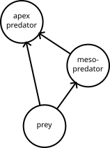
Figure 1. Example ecosystem
Label the three species:
- apex predator
- mesopredator
- prey
and let us assume the system obeys Lotka-Volterra dynamics with coefficience \(r\) and \(B\) defined below.
# Code is written in Python

import numpy as np
import matplotlib.pyplot as plt

# number of species
S = 3

# intrinsic growth rates
r = np.array([-0.09868652, -0.10491318,  1.24977311])

# Lotka-Volterra interaction terms
B = np.array(
    [
        [-8.28410720e-03,  2.81792972e-03,  1.11307405e-02],
        [-4.39125000e-05, -1.12271716e-03,  1.94991860e-02],
        [-6.15708830e-03, -5.27941320e-04, -2.51039475e-02]
    ]
)
At the steady state, the population sizes are:
n = np.linalg.inv(B) @ (-r)
print(n)
[100. 250. 20.]
The Jacobian evaluated at the steady state:
J = np.diag(n) @ B
print(J)
[[-0.82841072  0.28179297  1.11307405]
 [-0.01097812 -0.28067929  4.8747965 ]
 [-0.12314177 -0.01055883 -0.50207895]]
The eigenvalues of the Jacobian:
J_eigs = np.linalg.eigvals(J)
print(J_eigs)
[-0.99815469+0.j -0.30650713+0.52456685j -0.30650713-0.52456685j]
The maximum real part of the eigenvalues is negative, so the steady state is stable.
Let’s check if the eigenvalues of \(A\) match \(J\).
The scaled community matrix \(A\):
A = B @ np.diag(n)
print(A)
[[-0.82841072  0.70448243  0.22261481]
 [-0.00439125 -0.28067929  0.38998372]
 [-0.61570883 -0.13198533 -0.50207895]]
\(A\)’s eigenvalues are
A_eigs = np.linalg.eigvals(A)
print(A_eigs)
[-0.99815469+0.j -0.30650713+0.52456685j -0.30650713-0.52456685j]
So we have verified that \(A\) has the same eigenvalues as \(J\).
Check that scaling the dynamics works
Let us verify that the dynamics described by \(B\) and by \(A\) are the same.
We will start both systems with population sizes 1/10 of their value at steady state, and track how the population sizes change over time.
First, let’s do the original Lotka-Volterra system:
from scipy import integrate

# define the original dynamics
def dn_dt(n_t, t=0):
    return n_t * (r + B @ n_t)

# time range to plot the dynamics over
t = np.linspace(0, 20, 100)

# initial values for the population sizes
n_t_0 = 0.1 * n

# integrate numerically
n_t, infodict = integrate.odeint(dn_dt, n_t_0, t, full_output=True)
print(infodict["message"])

# plot
plt.plot(t, n_t, label=["apex", "meso", "prey"])
plt.title('Using B')
plt.xlabel('Time')
plt.ylabel('Unscaled population sizes')
plt.legend(loc="best")
plt.show()
Integration successful.
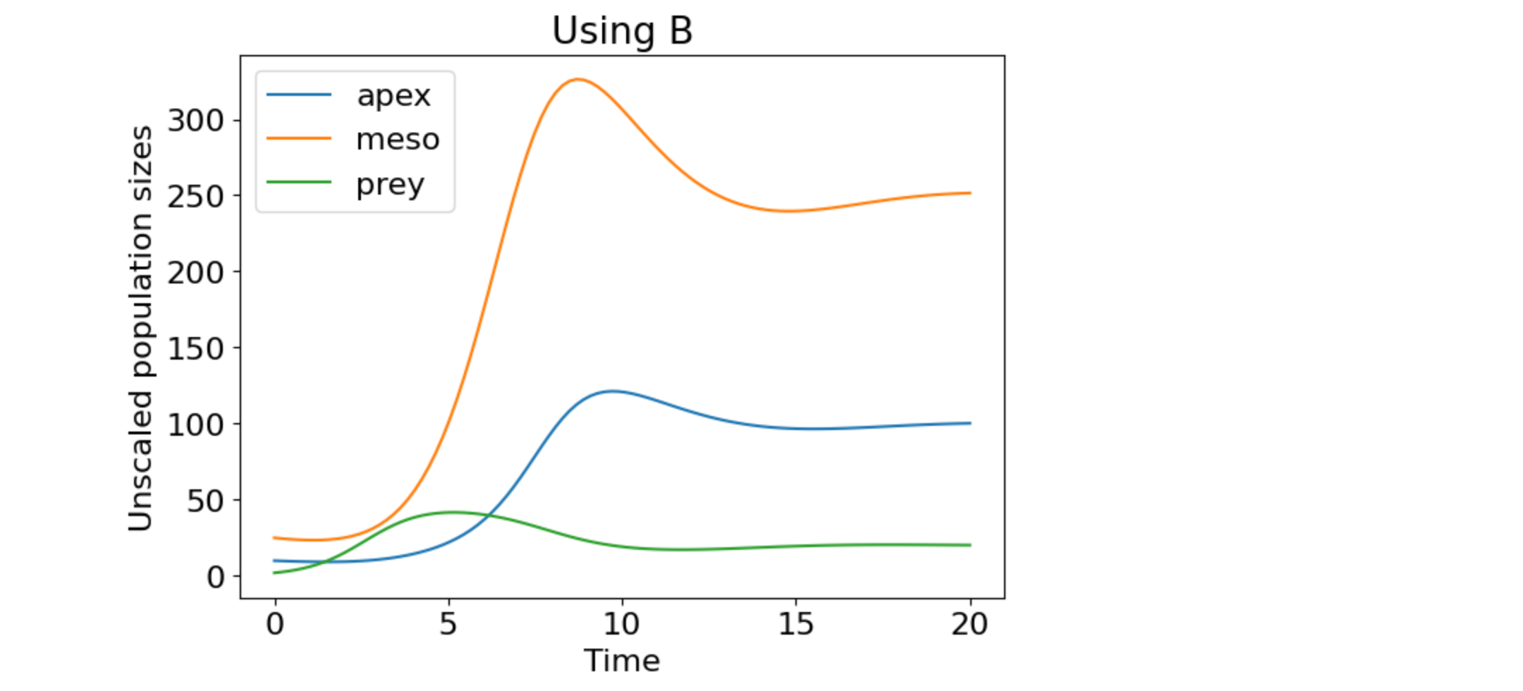
Figure 2. Ecosystem dynamics of the original, unscaled system.
We want to compare to scaled results, so let’s scale the plot by dividing through by the steady-state population sizes:
plt.plot(t, n_t/n, label=["apex", "meso", "prey"])
plt.title('Using B')
plt.xlabel('Time')
plt.ylabel('Scaled population sizes')
plt.legend(loc="best")
plt.show()
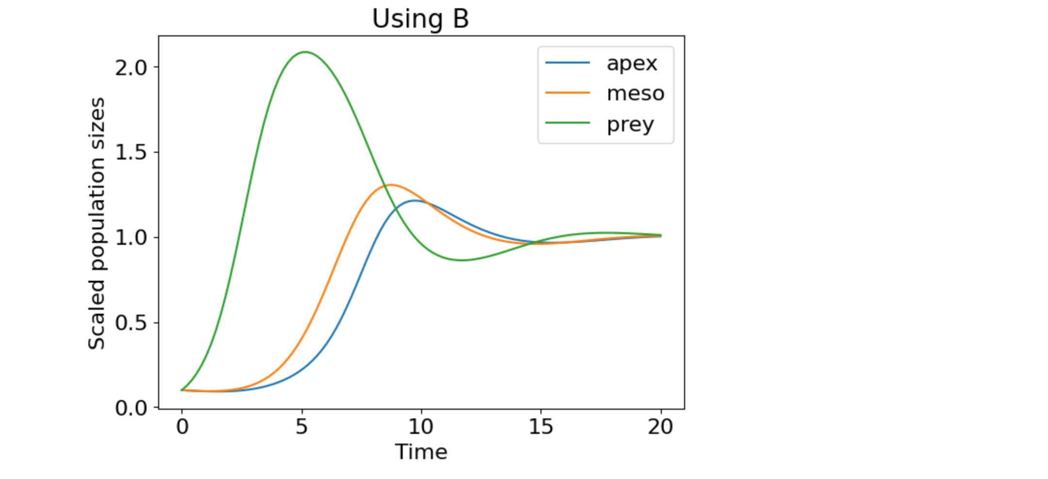
Figure 3. A repeat of Fig. 2 but the population sizes have been scaled to their steady-state values.
Now let’s do the dynamics of the scaled Lotka-Volterra system using the community matrix \(A\):
# define the scaled dynamics
def dx_dt(x_t, t=0):
    return x_t * (r + A @ x_t)

# initial values for the population sizes
x_t_0 = 0.1 * np.ones(3)

# integrate numerically
x_t, infodict = integrate.odeint(dx_dt, x_t_0, t, full_output=True)
print(infodict["message"])

# plot
plt.plot(t, x_t, label=["apex", "meso", "prey"])
plt.title('Using A')
plt.xlabel('Time')
plt.ylabel('Scaled population sizes')
plt.legend(loc="best")
plt.show()
Integration successful.
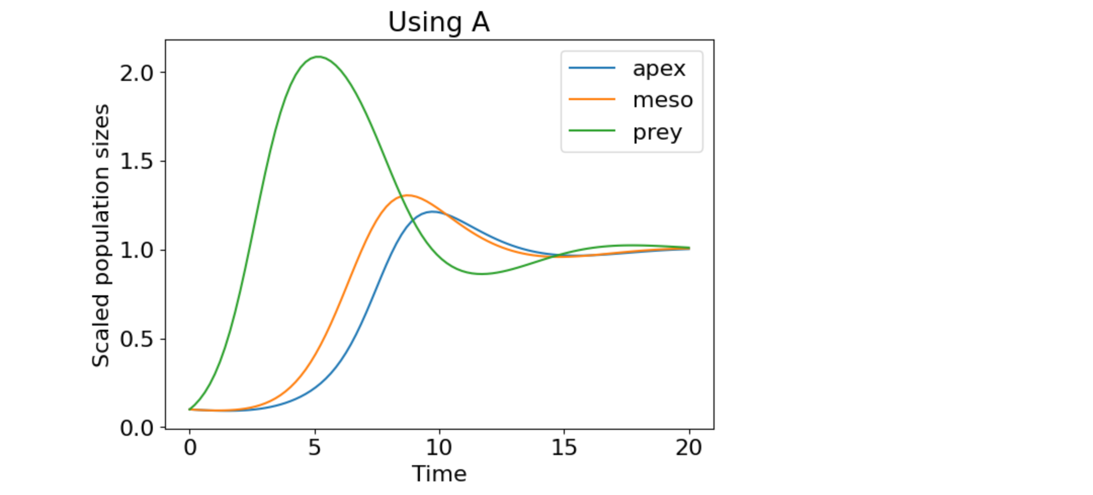
Figure 3. Ecosystem dynamics using the scaled matrix A.
Figs. 2 and 3 are the same, which verifies that the scaling preserves the dynamics.
Check method for species eradication works
Let’s now check that our equation for \(\delta_i\) (Eq. 15) is correct. First, let’s remove a species in the original system and see how it changes the population steady states. Then, let’s see if we can obtain the same proportional changes from the scaled community matrix alone. Let us remove the apex predator, species 1.
Our old interaction matrix and intrinsic growth rates were:
print("B = ")
print(B)
print("\nr = ")
print(r)
B =
[[-8.28410720e-03  2.81792972e-03  1.11307405e-02]
 [-4.39125000e-05 -1.12271716e-03  1.94991860e-02]
 [-6.15708830e-03 -5.27941320e-04 -2.51039475e-02]]

r =
[-0.09868652 -0.10491318  1.24977311]
When we remove the apex predator, our \(B_{i \neq 1, j \neq 1}\) and \(r_{i \neq 1}\) will be:
B_rem = B[1:S, 1:S]
print("new B = ")
print(B_rem)

# Note: Python indexes elements from 0, while Matlab indexes from 1.
# If you were to do this in Matlab, you'd do something like
#   B_rem = B(2:S, 2:S)

r_rem = r[1:S]
print("\nnew r = ")
print(r_rem)
new B =
[[-0.00112272  0.01949919]
 [-0.00052794 -0.02510395]]

new r =
[-0.10491318  1.24977311]
Therefore, the new population steady state is:
p = np.linalg.inv(B_rem) @ (-r_rem)
print(p)
[564.8740935 37.90450627]
And the proportional changes in the other species steady-state population sizes is:
delta = (p - n[1:S]) / n[1:S]
print("Proportional change from original Lotka Volterra equations:")
print(delta)
Proportional change from original Lotka Volterra equations:
[1.25949637 0.89522531]
We find that, when the apex predator is eradicated, both the meso-predator’s and prey’s population size increases.
Can we get the same \(\delta\) using Eq. 15 above? Let’s try.
Recall Eq. 15 says: \(\delta = (A_{i \neq k, j \neq k})^{-1} \; A_{i \neq k, k}.\)
Recall our \(A\) was:
print(A)
[[-0.82841072  0.70448243  0.22261481]
 [-0.00439125 -0.28067929  0.38998372]
 [-0.61570883 -0.13198533 -0.50207895]]
So \(A_{i \neq k, j \neq k}\) is:
A_rem = A[1:S, 1:S]
print(A_rem)
[[-0.28067929  0.38998372]
 [-0.13198533 -0.50207895]]
And \(A_{i \neq k, k}\) is:
A_col = A[:, 0][1:S]
print(A_col)
[-0.00439125 -0.61570883]
Applying Eq. 15:
delta_eq_15 = np.linalg.inv(A_rem) @ A_col
print("Proportional change from Eq 15:")
print(delta)
Proportional change from Eq 15:
[1.25949637 0.89522531]
Both methods give the same \(\delta\), which verifies Eq. 15 is correct.
References
Bender, E. A., Case, T. J. and Gilpin, M. E. (1984). Perturbation experiments in community ecology: theory and practice, Ecology 65(1): 1–13.
Kristensen, N.P., Chisholm, R.A., McDonald-Madden, E. (2019) Dealing with high uncertainty in qualitative network models using Boolean analysis, Methods in Ecology and Evolution 10: 1048-1061
Nakajima, H. (1992). Sensitivity and stability of flow networks, Ecological Modelling 62(1): 123–133.
Raymond, B., McInnes, J., Dambacher, J. M., Way, S. and Bergstrom, D. M. (2011). Qualitative modelling of invasive species eradication on subantarctic Macquarie Island, Journal of Applied Ecology 48(1): 181–191.