Group nepotism and the Brothers Karamazov Game
I recently read a classic paper by anthropologist Jones (2000), ‘Group nepotism and human kinship’, which argues that collective action may explain some of the key features of human cooperation between kin. Collective action here is action by a group (e.g., clan, tribe) that has sufficient ingroup solidarity to decide how to act as a collective. The key features it may help explain are: 1. the ‘axiom of amity’, that one is obliged to help kin just because they’re kin; 2. that kin groups come in many sizes and can be quite large; and 3. that human notions of kinship can be very different from biological kinship, sometimes occurring between individuals with no known geneological relationship.
The paper gives many detailed examples and arguments for why real-world social kinship has the features we would expect if group nepotism — combining relatedness with collective action — was an important mechanism (and also a section on ethnocentrism), which I cannot do justice here. Instead, the purpose of this blog post is to simply to teach myself about the basic idea by working through the first model in the paper.
Model background
The first model is called the Brothers Karamazov Game, named after the Dostoevsky novel. I’ve never read The Brothers Karamazov, but I gather there are three brothers — Ivan, Alyosha, and Dmitri — and Dmitri is prone to making poor life choices. The question is, should Ivan and Alyosha help out their brother Dmitri?
When Ivan and Alyosha act independently, then the rule for helping Dmitri to a benefit \(B\) at a cost \(C\) follows directly from Hamilton’s rule. The coefficient of relatedness between full siblings is \(r=1/2\); therefore, Ivan (or Alyosha) should help Dmitri if the benefit to Dmitri is at least twice the cost, \(B/C > 1/r = 2\). However, Jones shows this constraint can be made much easier to overcome if Ivan and Alyosha act together.
Jones introduces a situation he calls “conditional nepotism”: Ivan proposes to Alyosha that he will help out Dmitri if and only if Alyosha agrees to do the same. If Alyosha agrees to this, then when we add up Ivan’s inclusive fitness costs and benefits (details below), the pooling of nepotistic effort leads for a condition for helping \(B/C > 1/r_c\) where \(r_c > r\). In other words, provided Alyosha agrees, then Ivan should treat Dmitri as though he is even more related to him than he really is. This is an interesting result because it might help explain why helping between kin — culturally defined — is common in hunter-gatherer societies even though relatedness coefficients between pairs of individuals are often quite low.
Approach
I will now work through the sexual haploid case in the first appendix. However, instead of using Jones’ method, I will try performing the calculations using the framework provided in Ohtsuki (2014; Proc R Soc B).
Ohtsuki’s method allows us to describe the replicator dynamics of two strategies \(A\) and \(B\) in nonlinear games played between kin by taking into account the higher-order genetic associations between group members, beyond their dyadic relatedness. Dyadic relatedness \(r\) above is the probability that 2 individuals randomly drawn without replacement from the group will have strategies that are identical by descent, denoted \(\theta_{2 \rightarrow 1}\) in Ohtsuki’s scheme. We can also say in shorthand that the two individuals “share a common ancestor”. Higher-order relatedness generalises this concept to larger samples. For example, \(\theta_{3 \rightarrow 1}\) is the probability that three individuals randomly drawn share a common ancestor, and in general, \(\theta_{l \rightarrow m}\) is the probability that, if we draw \(l\) individuals from the group, they share \(m\) common ancestors.
The higher-order genetic associations \(\theta_{l \rightarrow m}\) can then be used to find the probilities \(\rho_l\) that \(l\) players randomly sampled from the group without replacement are \(A\)-strategists (Eq. 2.5):
\[\rho_l = \sum_{m=1}^l \theta_{l \rightarrow m} p^m\]where \(p\) is the proportion of \(A\)-strategists in the population and \(\rho_0=1\).
The reasoning behind the \(\rho_l\) equation can be seen by considering the probability that two randomly sampled group members are \(A\)-strategists, \(\rho_2\). Either the two individuals have the same ancestor, or they have different ancestors. Assuming that the proportion of \(A\)-strategists in the ancestral population can be approximated by the proportion of \(A\)-strategists now, then:
\[\rho_2 = \quad \underbrace{\theta_{2 \rightarrow 1}}_{\substack{\text{same} \\ \text{ancestor}}} \quad \underbrace{p}_{\substack{\text{ancestor} \\ \text{=A}} } \quad + \quad \underbrace{\theta_{2 \rightarrow 2}}_{\substack{\text{two} \\ \text{ancestors}} } \quad \underbrace{p^2}_{\substack{\text{both} \\ \text{=A}}}\]Let’s define the payoffs to the two strategies using two functions: \(a_k\) is the payoff to \(A\)-strategists when \(k\) of the \(n-1\) other group members are \(A\)-strategists, and \(b_k\) is the payoff to \(B\)-strategists when \(k\) of the \(n-1\) other group members are also \(A\)-strategists.
Then Ohtsuki (2014) shows that the change in the proportion \(A\)-strategists in the population, \(p\), over one generation is proportional to (Eq. 2.4)
\[\Delta p \propto \sum_{k=0}^{n-1} \sum_{l=k}^{n-1} (-1)^{l-k} {l \choose k} {n-1 \choose l} \left[ (1-\rho_1) \rho_{l+1} a_k - \rho_1(\rho_l - \rho_{l+1}) b_k \right].\]This equation is derived from first principles from the Price equation (see Ohtsuki (2014) appendices).
Results
Dynamics equation
The number of terms in the dynamics equation quickly becomes unweildy, so I’ll use SageMath below to work through the algebra.
First, I will prepare the symbolic function “\(\Delta p \propto \ldots\)”
%display latex

var('B, C') # benefit and cost of helping behaviour
n = 3       # size of the group (3 brothers)

# a placeholder for the payoff functions a_k and b_k we'll define later
a = function('a')
b = function('b')

# a placeholder for the rho function we'll define later
rho = function('rho')

var('l,k') # sum counters

# Eq. 2.4 from Ohtsuki (2014)
delta_pr = sum(sum((-1)^(l-k) * binomial(l, k) * binomial(n-1, l) * ( (1-rho(1))*rho(l+1)*a(k) - rho(1)*(rho(l)-rho(l+1))*b(k) ), l, k, n-1), k, 0, n-1)
delta_prThe example in Section 4(b) of Ohtsuki (2014) provides us with expressions for the higher-order relatedness terms between siblings. Define the dyadic relatedness \(r = \theta_{2 \rightarrow 1}\) as before, and define the triplet relatedness \(s = \theta_{3 \rightarrow 1}\). Then it can be shown:
\[\begin{align} \theta_{1 \rightarrow 1} &= 1, \\ \theta_{2 \rightarrow 1} &= r, \\ \theta_{2 \rightarrow 2} &= 1-r, \\ \theta_{3 \rightarrow 1} &= s, \\ \theta_{3 \rightarrow 2} &= 3r - 3s, \\ \theta_{3 \rightarrow 3} &= 1 - 3r + 2s. \end{align}\]Between siblings, \(r = 1/2\) and \(s = 1/4\), therefore
\[\begin{align} \rho_1 &= \theta_{1 \rightarrow 1} p = p, \\ \rho_2 &= \theta_{2 \rightarrow 1} p + \theta_{2 \rightarrow 2} p^2 = \frac{p}{2} + \frac{p^2}{2}, \\ \rho_3 &= \theta_{3 \rightarrow 1} p + \theta_{3 \rightarrow 2} p^2 + \theta_{3 \rightarrow 3} p^3 = \frac{p}{4} + \frac{3p^2}{4} \end{align}\]We will substitute these expressions for \(\rho_l\) into the symbolic function:
var('p')
delta_pr = delta_pr.subs({
    rho(0): 1,
    rho(1): p,
    rho(2): p/2 + p^2/2,
    rho(3): p/4 + 3*p^2/4,
})
delta_prNow we have an expression proportional to \(\Delta p\) to which we can apply different payoff functions \(a_k\) and \(b_k\).
Unconditonal helping vs. defection
First, let’s consider the case where the two brothers always help Dmitri regardless of what the other does. We already know the answer whether or not this behaviour can evolve, it follows directly from Hamilton’s Rule, so this also serves to sanity-check the calculations.
Let the \(A\) strategy be unconditional helping and \(B\) be defection. When the focal player is playing the role of Dmitri, which is drawn with probability \(1/3\), their payoffs are independent of their strategy
\[\begin{pmatrix} a_0 & a_1 & a_2 \\ b_0 & b_1 & b_2 \end{pmatrix} = \begin{pmatrix} 0 & B & 2B \\ 0 & B & 2B \end{pmatrix}\]If the focal is not a Dmitri (occurs with probability 2/3), the payoffs to the focal depend on whether or not they help the Dmitri
\[\begin{pmatrix} a_0 & a_1 & a_2 \\ b_0 & b_1 & b_2 \end{pmatrix} = \begin{pmatrix} -C & -C & -C \\ 0 & 0 & 0 \end{pmatrix}\]Therefore, when the brothers act independently, the expected payoffs
\[\begin{pmatrix} a_0 & a_1 & a_2 \\ b_0 & b_1 & b_2 \end{pmatrix} = \frac{1}{3} \begin{pmatrix} -2C & B-2C & 2B-2C \\ 0 & B & 2B \end{pmatrix}\]Substituting these payoffs into the expression proportional to \(\Delta p\)
uncond_delta_pr = delta_pr.subs({
    a(0): -2*C/3,
    a(1): B/3 - 2*C/3,
    a(2): 2*B/3 - 2*C/3,
    b(0): 0,
    b(1): B/3,
    b(2): 2*B/3
})
uncond_delta_pr = uncond_delta_pr.expand().factor()
uncond_delta_prThe condition for the \(A\)-strategist (the ones who help Dmitri) to increase is
\[B-2C > 0\]and the condition is
\[B/C > 2 = 1/r\]as expected.
Conditional nepotism vs. defection
Now let’s consider Jones’ scenario, where Ivan and Alyosha help Dmitri if and only if they both agree, i.e., they are both conditional nepotists.
You might notice in the first appendix that Jones talks about a ‘conditional nepotists’ vs ‘Hamiltonian nepotists’ scenario, which confused me at first, because when you look at the payoffs Table A2, there’s no helping by the Hamiltonian \(H\) type. I think what’s happening is he is actually restricting his attention to the situation \(B/C < 2\), and assuming that what he calls ‘Hamiltonian nepotists’ will decide to not help Dmitri in this situation, i.e., act like defectors (see wording of the paragraph right after Eq. A1). Therefore, the scenario in question is actually ‘conditional nepotists vs defectors’. Hopefully this will become clear by the time we’ve gone through all the cases (final figure summary).
Let the \(A\) strategy be conditional nepotism and the \(B\) strategy be defection. When the focal player is a Dmitri (probability \(1/3\)), their payoffs are again independent of their strategy
\[\begin{pmatrix} a_0 & a_1 & a_2 \\ b_0 & b_1 & b_2 \end{pmatrix} = \begin{pmatrix} 0 & 0 & 2B \\ 0 & 0 & 2B \end{pmatrix}\]When the focal player is not a Dmitri (probability 2/3), their payoffs are
\[\begin{pmatrix} a_0 & a_1 & a_2 \\ b_0 & b_1 & b_2 \end{pmatrix} = \begin{pmatrix} 0 & -C/2 & -C \\ 0 & 0 & 0 \end{pmatrix}\]where \(a_1 = -C/2\) because, if there is one other helper in the group, there is half a chance that the other helper is also not a Dmitri and thus the \(A\)-strategist gives the help.
Therefore, when the brothers act as conditional nepotists, the expected payoffs
\[\begin{pmatrix} a_0 & a_1 & a_2 \\ b_0 & b_1 & b_2 \end{pmatrix} = \frac{1}{3} \begin{pmatrix} 0 & -C & 2B-2C \\ 0 & 0 & 2B \end{pmatrix}\]cond_delta_pr = delta_pr.subs({
a(0): 0,
a(1): -C/3,
a(2): 2*B/3 - 2*C/3,
b(0): 0,
b(1): 0,
b(2): 2*B/3
})
cond_delta_pr = cond_delta_pr.expand().factor()
cond_delta_prThe condition for conditional nepotists to increase matches the equation that Jones presents in the appendix (Eq. A1)
\[2Bp - 2Cp + B - 2C > 0\]or
\[\frac{B}{C} > \frac{2 + 2p}{1 + 2p} \equiv \frac{1}{r_c}.\]As \(p\) increases from 0 to 1, \(r_c\) above increases from 1/2 to 3/4, meaning that when \(p\) is high, the brothers will treat Dmitri as though he is more related to them than he really is. Conditional nepotists can invade defectors when (sub in \(p=0\)) \(B/C > 2\). Defectors can invade conditional nepotists (sub in \(p=1\), reverse condition) when \(B/C < 4/3\).
Let’s plot some examples of the \(\Delta p\) vs \(p\) function to get a more intuitive feel. When \(B/C = 2.5 > 2\), we see below that \(\Delta p\) is always greater than zero.
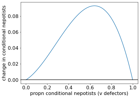
Change in proportion of conditional nepotists when (B/C = 2.5)
When \(B/C = 1.5\) (satisfying \(4/3 < B/C < 2\)), we see that \(\Delta p\) is less than zero when \(p\) is small, and greater than zero when \(p\) is large. There are two stable steady states — all Defectors and all Conditional Nepotists — and a separatrix between them. The position of the separatrix is found by setting the \(B/C\) condition above to an equality: \(p^{\star} = \frac{2C-B}{2B-2C}\).
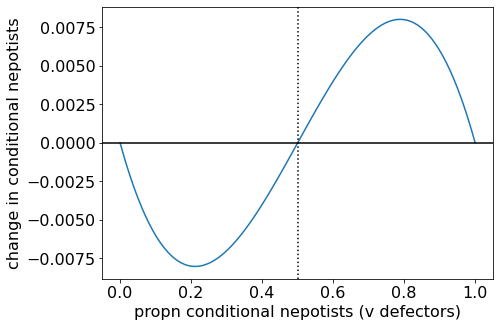
Change in proportion of conditional nepotists when (B/C = 1.5).
When \(B/C = 1.2 < 4/3\), \(\Delta p\) is always below zero. All-defectors is the evolutionary endpoint.
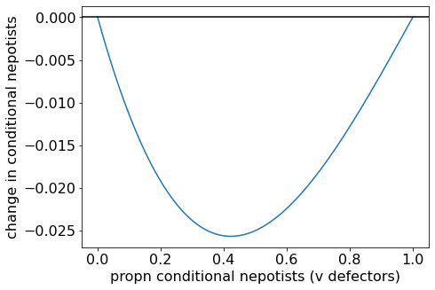
Change in proportion of conditional nepotists when (B/C = 1.2).
Conditional nepotism vs. unconditional helping
For completeness, we should now consider the case of ‘conditional nepotists’ vs ‘unconditional helpers’. Let the \(A\) strategy be conditional nepotism and the \(B\) strategy be unconditional helping. Substituting in the expected payoffs:
x_delta_pr = delta_pr.subs({
    a(0): (2*B)/3,
    a(1): (B-C)/3,
    a(2): (2*B-2*C)/3,
    b(0): (2*B-2*C)/3,
    b(1): (B-2*C)/3,
    b(2): (2*B-2*C)/3
})

x_delta_pr = x_delta_pr.expand().factor()
x_delta_prThe condition for conditional nepotists to increase is
\[B(2p-1) > C(2p-2)\]which splits up into two cases. When \(p > 1/2\), the condition becomes
\[\frac{B}{C} > \frac{2p-2}{2p-1}\]and so conditional nepotists can always grow. When \(p < 1/2\), the condition becomes
\[\frac{B}{C} < \frac{2p-2}{2p-1}\]and conditional nepotists can only invade (\(p=0\)) if \(B/C < 2\).
Let’s again plot some examples to obtain the intuition. First, let’s plot an example where \(B/C < 2\). The \(p^*=0\) steady state is unstable, \(p^* =1\) is stable, and there are no interior equilibria. Therefore, conditional nepotists can invade, and an all-conditional-nepotists population is the evolutionary endpoint.
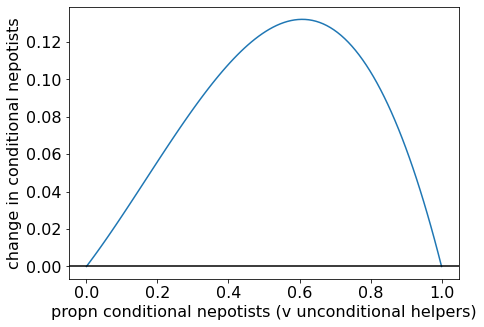
Change in proportion of conditional nepotists when (B/C = 1.5).
Now let’s see how the situation changes as we move to the \(B/C > 2\) space. In the plot below, we see how, when we reach \(B/C = 2\), an interior separatrix appears, so now there are two evolutionarily stable states: all conditional nepotists, and all unconditional helpers. So conditional nepotists cannot invade, but once established, they can resist invasion by unconditional helpers.
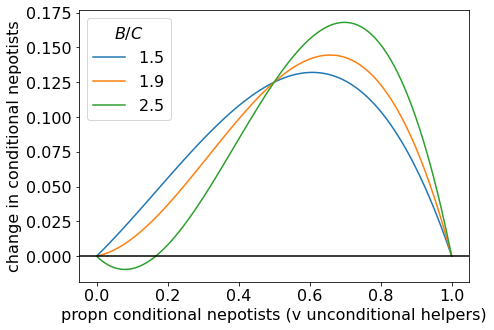
Change in proportion of conditional nepotists for a range of (B/C) values.
As \(B/C\) becomes larger, the separatrix moves to the right. When we plot an example with large \(B/C\), the separatrix is close to \(p \approx 1/2\), as suggested above.
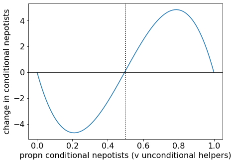
Change in proportion of conditional nepotists for (B/C = 100).
Summary of dynamics
All evolutionary endpoints are monomorphic, so I summarised the evolutionary dynamics in terms of pairwise invasibility below.
When benefits are high compared to costs, defectors cannot prevail. The evolutionary endpoints are conditional nepotists or unconditional helpers. When benefits are intermediate \(4/3 < B/C < 2\), unconditional helpers are no longer evolutionarily stable. Either defectors or conditional nepotists will prevail. When benefits are low, defectors prevail.
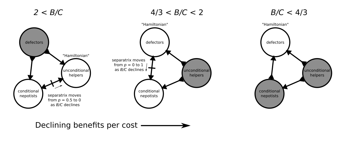
A summary of the evolutionary dynamics of the Brothers Karamazov game across three regimes determined by the cost-benefit ratio. White circles indicate evolutionary endpoints, directions of arrows indicate whether populations are resistant to invasion or invasible, and solid lines on edges indicate separatrices.
Conditional nepotists can never invade. However, if the benefits are close to but just above \(B/C = 2\), the separatrix between conditional nepotists and unconditional helpers is close to zero. This suggests that, if a cluster of unconditional helpers have a brainwave and strike upon the idea of making a deal like Jones describes, then they might be able to invade and explore the new space of potential collaborative situations not previously accessible to the unconditional helpers. The separatrix between conditional nepotists and defectors is near 0 when \(B/C\) is near \(2\), so they will (at least, initially), be quite resistant to invasion by defectors.
Conclusion
The Brothers Karamazov model above is only the first of 3 models that Jones (2000) discusses. In the second model, Jones considers a large donor group facing the choice of whether to help another group of relatives. Through a similar principle to “conditional nepotism” above, the donor group decides as a collective whether or not to help, i.e., “group nepotism”. Analogous to \(r_c\) above, “group coefficient of relatedness” \(r_g\) is obtained from the condition \(B/C > 1/r_g\), and it too can be larger than dyadic relatedness \(r\).
Table 1 below compares estimates of the dyadic relatedness (labelled \(r_{11}\) in the talbe) and the group coefficient of relatedness for a sampling of tribal societies. Group relatedness is often much higher than dyadic relatedness, sometimes nearing 1. This suggests that, if groups of relatives can somehow coordinate themselves and act as a collective, then they will render help more easily than one would expect just from individual inclusive fitness considerations alone.

Jones proposes that such collective behaviour might be achieved by “mutual coercion, mutually agreed upon”, and gives many real-life anthropological examples where individuals are punished for not obeying norms about how one ought to treat their (culturally defined) kin. Models that also include coercion (punishment) could be used to learn more about the exact conditions under which this can evolve. So I have more reading to do.
Further reading
Jones, D. (15 June, 2016). Blog post: “Beating Hamilton’s Rule”, https://logarithmichistory.wordpress.com/2016/06/15/beating-hamiltons-rule/
References
Jones, D. (2000). Group nepotism and human kinship. Current Anthropology, 41(5): 779-809
Ohtsuki, H. (2014). Evolutionary dynamics of n-player games played by relatives. Philosophical Transactions of the Royal Society B: Biological Sciences, 369(1642), 20130359.