Connection between replicator dynamics, Bernstein polynomials, and Bezier curves
A series of papers by Jorge Peña and others provide a neat way to characterise the replicator dynamics of two-strategy nonlinear public goods games with random group formation (Peña et al. 2014, Peña et al. 2015, Peña & Nöldeke 2016, Nöldeke & Peña 2016, Peña & Nöldeke 2018, Nöldeke & Peña 2020). I this blog post, I used a paper by Archetti (2018) to teach myself more about the topic.
Archetti (2018) considered replicator dynamics in a population of producers (cooperators) and defectors. The probability that \(i\) of the \(n-1\) other members in your group are cooperators is
\[p_{i,n-1}(x) = { n-1 \choose i } x^i (1-x)^{n-1-i}\]where \(x\) is the proportion of cooperators in the population. The fitnesses of cooperators and defectors are
\[\begin{align} W_C &= \sum_{i=0}^{n-1} p_{i,n-1}(x) b(i+1) - c, \\ W_D &= \sum_{i=0}^{n-1} p_{i,n-1}(x) b(i), \end{align}\]respectively, where \(b(i)\) is the benefit from the public good and \(c\) is the cost of contributing. The cooperator gets \(b(i+1)\) to count themselves. The replicator dynamics are
\[\dot{x} = x(1-x) \beta(x) \label{dotx}\]where
\[\beta(x) = \sum_{i=0}^{n-1} p_{i,n-1}(x) \Delta b_i, \quad \text{and} \quad \Delta b_i = b(i+1) - c - b(i).\]The \(\Delta b_i\) are also the change in payoff from switching strategy.
The steady states are found when \(\dot{x} = 0\). There are two trivial steady states, \(x^*=0\) and \(x^*=1\). Any additional steady states are found by finding the roots \(\beta(x)=0\). When \(b(i)\) is nonlinear, it can be difficult to solve \(\beta(x) = 0\) analytically.
Archetti (2018) explain how the general shape of \(\beta(x)\) can be determined by harnessing the theory of Bernstein Polynomials. A Bernstein polynomial basis of degree \(n\) for \(x = [0,1]\) is
\[p_{i,n}(x) = {n \choose i} x^i (1-x)^{n-i}\]A polynomial in Bernstein form is
\[F(x) = \sum_{i=0}^n p_{i,n}(x) f_i \label{F(x)}\]where \(f_i\) is the Bernstein coefficient.
Comparing the equations above, it is apparent that \(\beta(x)\) is a polynomial in Bernstein form, and \(\Delta b_i\) is its Bernstein coefficients:
\[\underbrace{\beta(x) \vphantom{\sum_i^n} }_{F(x)} = \underbrace{\sum_{i=0}^{n-1}}_{\sum_{i=0}^n} \underbrace{p_{i,n-1}(x)\vphantom{\sum_i^n} }_{p_{i,n}} \underbrace{\Delta b_i\vphantom{\sum_i^n} }_{f_i} \nonumber\]Archetti (2018) provides a flexible function for \(b_i\), which can provide a variety linear and highly nonlinear games (e.g., sigmoid, step-function). The benefit \(b(i)\) from the public good to an individual in a group with \(i\) producers and \((n - i)\) defectors is
\[b(i) = \frac{l(i) - l(0)}{l(n) - l(0)}, \quad \text{ where } \quad l(i) = \frac{1}{1 + e^{s(h - i/n)}}.\]Some examples
Consider a game parameterised with \(s = 10\), \(h = 0.4\), \(c = 0.05\). This produces a sigmoid relationship between the number of cooperators and the benefit from the public good. Their Fig. 5 shows how the Bernstein coefficients \(\Delta b_i\) compare to \(\beta(x)\). Please note that I wasn’t able to reproduce their Fig. 5 exactly, but I will provide all the details so anyone can find where the issue might have been.
Start with the simplest example, \(n=2\). Substituting the parameters into the equations for \(l(i)\) and \(b(i)\) above, I obtained
\[l(0) = 0.018, \quad l(1) = 0.731, \quad l(2) = 0.998, \quad b(0) = 0, \quad b(1) = 0.728, \quad b(2) = 1\]The Bernstein coefficient \(\Delta b_i = b(i+1) - c - b(i)\), which results in:
\[\Delta b_0 = 0.678, \quad \Delta b_1 = 0.222. \label{two_only}\]Any interior equilibria are found as the roots of
\[\beta(x) = \sum_{i=0}^{n-1} { n-1 \choose i } x^i (1-x)^{n-1-i}\]which, for \(n=2\), results in the linear equation
\[\beta(x) = \Delta b_0 + x(\Delta b_1 - \Delta b_0),\]with endpoints:
\[\beta(x=0) = 0.678, \quad \beta(x=1) = 0.222.\]Fig. 1 compares \(\Delta b_i\) and \(\beta(x)\), and the two lines lie on top of each other. The reason for this is because, when \(n\) is only 2, \(\beta(x)\) is linear, and also because of the endpoints property of Bernstein polynomials:
The initial and final values of \(f\) and \(F\) are the same: \(F(0) = f_0\); \(F(1) = f_n\).
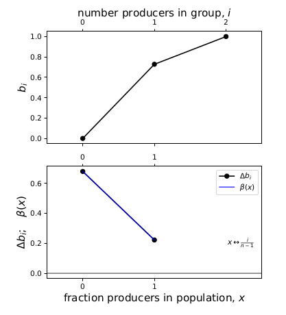
Figure 1: Comparing the linear spline formed of the Bernstein coefficients and beta(x) for n=2.
We know that in two-strategy two-player games with replicator dynamics, the Nash Equilibria are equivalent to the replicator stable steady states, and the coefficients are the change in payoff from switching strategies.
Fig. 2 compares \(\Delta b_i\) and \(\beta(x)\) for a variety of \(n\). Two interesting properties are illustrated here. First, the \(\Delta b_i\) linear spline preserves the shape of \(\beta(x)\). Across these examples and the additional ones in Archetti (2018), we find that when \(\beta(x)\) is convex, concave, or monotone, the \(\Delta b_i\) linear spline is likewise convex, concave, or monotone.
The second interesting property is that, as \(n\) increases, the agreement between \(\Delta b_i\) and \(\beta(x)\) improves. This is another property of Bernstein polynomials: the coefficients are an approximation of the continuous function, which improves as \(n \rightarrow \infty\).
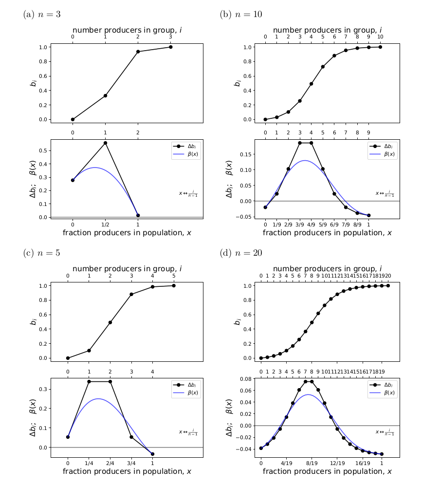
Figure 2: Comparing the linear spline formed of the Bernstein coefficients and beta(x) for higher n.
An intuitive way to understand the shape-preserving and convergence properties is by understanding that the Bernstein polynomial is a Bezier curve and the coefficients are the control points. Below is an animation of a Bezier curve with 3, 4, and 5 control points from its Wikipedia page.
Fig. 4 shows how \(\beta(x)\) is drawn as a Bezier curve using the \(\Delta b_i\) as control points.
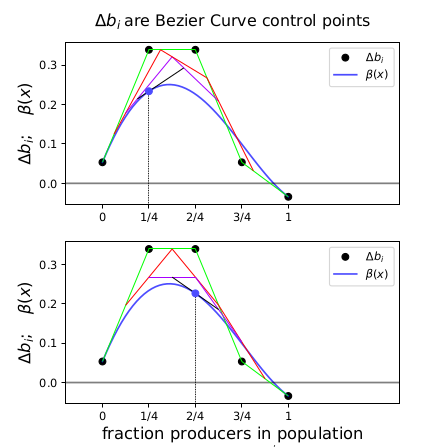
Figure 4: Drawing the n=5 Bezier curve at x=1/4 and x=1/2.
Characterising the dynamics
On page 5, Archetti (2018) detail how the Bernstein approach can be used to characterise the dynamics of the sigmoid game above. An important point to note is that finding the interior equilibria, i.e., the roots \(\beta(x)\), cannot be done from \(\Delta b_i\) alone (i.e., their first two bullet points involving conditions on \(\beta_{\text{MAX}}\)). A small example illustrates.
Consider the same game above, with \(n=10\), but now we increase the cost of contribution \(c\) from 0.05 to \(c=0.2\). In effect, this shifts the axis up and places it between the two curves. Fig. 5 compares the \(\Delta b_i\) spline to \(\beta(x)\). In this case, the spline has two interior roots but \(\beta(x)\) has none.
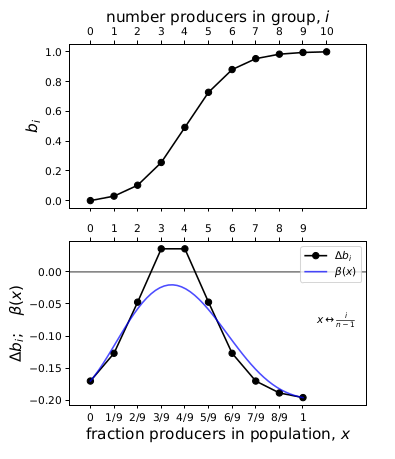
Figure 5: An example where the Bernstein coefficients suggest interior roots but beta(x) does not have interior roots.
It seems to me that the non-existence of roots of the \(\Delta b_i\) spline might tell you about the non-existence of interior equilibria in this case, but not the reverse. Perhaps this might be true for convex and concave pairs of roots in general, if I understand the shape-preserving property correctly.
Three or more strategies
Towards the end of the paper, Archetti (2018) write that nonlinearities are clearly important for games with more than two strategies, but analysis remains problematic for these games.
One generalisation of the Bernstein approach that would suit replicator dynamics is the Bernstein polynomial on the simplex. Its basis is the multinomial distribution (see, e.g., Definition 1 from Bayad et al. (2011)). The coefficients preserve axial convexity, which means the function is convex in any direction parallel to the edges of the simplex (Dahmen 1991, Sauer 1991).
The replicator dynamics of an \(m\)-strategy game can be put into Bernstein polynomial form. Index the strategies \(s_1, \ldots, s_{m}\) with payoffs \(\pi_{i}(\mathbf{k})\) to a focal \(s_i\)-strategist, where \(\mathbf{k} = [k_{1}, k_{2}, \ldots, k_{m}]\) is the total number of group members (i.e., including the focal player) with strategies \(s_1, s_2, \ldots, s_m\). Let \(\mathbf{p} = [p_1, \ldots, p_m]\) be the proportions of different strategists in the population. Let \(\mathbf{e_i}\) be a vector with 1 in position \(i\) and 0 elsewhere.
Define the set of all possible group compositions
\[K = \left\{ \mathbf{k} \, \middle\vert \, \sum_{j=1}^m k_{j} = n \right\}.\]Then the dynamics of \(x\)-strategists is proportional to
\[\Delta p_x \propto p_x \underbrace{\sum_{\mathbf{k} \in K} \underbrace{ \vphantom{ \sum_{i=1}^m } P(\mathbf{k} \mid n, \mathbf{p})}_{\text{Bernstein basis}} \underbrace{ \left( \sum_{i=1}^{m} k_{i} ( \pi_{x}(\mathbf{k} - \mathbf{e}_i + \mathbf{e}_x) - \pi_{i}(\mathbf{k}) ) \right) }_{\text{Bernstein coefficient}}.}_{\beta} \label{interior_bernstein}\]Again we see that the Bernstein coefficient is related to the change in payoffs when an individual switches strategy, which provides some kind of connection to the NE.
An example
Sigmund et al. (2010) modelled evolution by social learning in a PGG with a variety of different punishment regimes. They showed that, when punishment was implemented via an institution that punished both non-contributors to the PGG as well as non-contributors to the institution (e.g., non-payers of tax), then cooperation could be sustained.
I included only three of the types from their model, excluding the ‘loner’ type that is needed for punishers to invade.
(1) Cooperators (\(x\)), who contribute to the public good but not to the punishment pool, have payoff
\[\pi_x = \frac{r c (k_x + k_v) }{n-1}- c - B k_v.\](2) Defectors (\(y\)), who don’t contribute to anything, have payoff
\[\pi_y = \frac{r c (k_x + k_v) }{n-1} - B k_v.\](3) Punishers (\(v\)), who contribute to both the public good and the punishment institution, have payoff
\[\pi_v = \frac{r c (k_x + k_v) }{n-1} - c - G.\]I used their default parameter values: \(n = 5, r = 3, c = 1, B = G = 0.7\).
Fig. 6 summarises the replicator dynamics of the model. As described in their paper, when the institution metes out both 1st and 2nd-order punishment, a population of punishers is stable. However, punishers cannot invade unless their initial population is above some certain threshold.
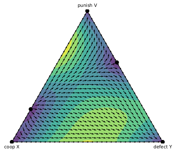
Figure 6: The replicator dynamics for the Sigmund model example. Created using egtsimplex
Fig. 7 compares the Bernstein coefficients to the full \(\beta\) function for the Sigmund model. The blue surface \(\beta\) matches the dynamics in Fig. 6 above, and the coefficients preserve the shape of \(\beta\). The two functions match at the endpoints (\(X=1\), \(Y=1\), \(V=1\)). Sigmund modelled an underlying linear game between cooperators and defectors, so \(\beta\) on the \(X\)-\(Y\) is linear and the line lies on top of the coefficients. Otherwise, the coefficients match the axial convexity in the directions parallel to the \(X\)-\(V\) and \(Y\)-\(V\) axes.
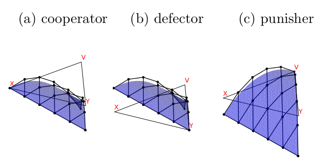
Figure 7: Comparing the linear mesh formed of the Bernstein coefficients (black) and the surface of the beta (blue) for the Sigmund model example. The flat triangle is the simplex axes where the coefficients and beta equal 0.
References
Archetti, M. (2018). How to analyze models of nonlinear public goods, Games 9(2): 17.
Bayad, A., Kim, T., Lee, S. H., & Dolgy, D. V. (2011). A note on the generalized Bernstein polynomials. Honam Mathematical Journal, 33(3), 431-439.
Dahmen, W. (1991). Convexity and Bernstein-Bézier polynomials, in P.-J. Laurent, A. Le Méhauté and L. L. Schumaker (eds), Curves and Surfaces, Academic Press, pp. 107–134.
Nöldeke, G. & Peña, J. (2016). The symmetric equilibria of symmetric voter participation games with complete information. Games and Economic Behavior, 99, 71–81.
Nöldeke, G. & Peña, J. (2020). Group size and collective action in a binary contribution game. Journal of Mathematical Economics, 88, 42–51.
Peña, J., Lehmann, L. & Nöldeke, G. (2014). Gains from switching and evolutionary stability in multi-player matrix games. Journal of Theoretical Biology, 346, 23–33.
Peña, J., Nöldeke, G. & Lehmann, L. (2015). Evolutionary dynamics of collective action in spatially structured populations. Journal of Theoretical Biology, 382, 122–136.
Peña, J., & Nöldeke, G. (2016). Variability in group size and the evolution of collective action. Journal of Theoretical Biology, 389, 72-82.
Peña, J., & Nöldeke, G. (2018). Group size effects in social evolution. Journal of Theoretical Biology, 457, 211-220.
Sauer, T. (1991). Multivariate Bernstein polynomials and convexity, Computer Aided Geometric Design 8(6): 465–478.
Sigmund, K., De Silva, H., Traulsen, A. and Hauert, C. (2010). Social learning promotes institutions for governing the commons, Nature 466(7308): 861.