Evolutionary game theory model with homophilic imitation
The purpose of this blog post is to replicate results from Vasconcelos et al. (2014) and use it to learn about the behaviour of this kind of model:
I am interested in this model because it involves homophily: it is a social learning model, but the probability of imitation depends not only on the relative payoffs between the focal player and other but also on how similar they are in wealth. Code can be found on Github: vasconcelos-2014-playground.
The model
Consider a population of \(Z\) individuals of which \(Z_R\) are rich and \(Z_P\) are poor. The rich and poor have different endowments, \(b_R > b_P\), from which they can contribute to a public goods game (PGG). Two strategies are possible. Cooperators contribute fraction \(c\) of their endowment to the PGG – so rich cooperators contribute \(c_R = c b_R\) and poor cooperators contribute \(c_P = c b_P\) – and defectors contribute nothing.
Individuals are randomly sampled into groups of size \(N\) to play the PGG. Let \(j_R\) be the number of rich cooperators in the group and \(j_P\) the number of poor cooperators (note a typo in Methods section). Therefore, there are \(N - j_R - j_P\) of defectors in the group, and the total contribution of the group is \(c_R j_R + c_P j_P\).
The game is a PGG with a threshold, which is set proportional to the average endowment. Let the average endowment \(\bar{b}\) satisfy \(Z \bar{b} = Z_R b_R + Z_P b_P\). In the paper, the default value \(\bar{b}=1\). The threshold is set \(M c \bar{b}\), where \(0 < M \leq N\), so it’s roughly a measure of how many cooperators are needed to pass the threshold.
Define \(\Delta\) as how far we are from the threshold \(\Delta = c_R j_R + c_P j_P - M c \bar{b}\). So a positive \(\Delta\) means the threshold was successfully met in the PGG. For convenience, define an indicator function to indicate if the group has met or exceeded the threshold: \(\Theta(\Delta) > 1\) if \(\Delta \geq 0\), otherwise 0.
When the threshold directly maps to the public-goods tasks outcome (i.e., under risk=1; see below), then the payoffs are calculated as follows.
For defectors, if the threshold is met, then they keep their endowment; otherwise, they lose it all. So the payoff for defectors is \(\Pi^D = b \Theta(\Delta)\).
For cooperators, if the threshold is met, then they keep what remains of their endowment after their contribution; otherwise, they lose it all. So the payoff for cooperators is \(\Pi^C = b \Theta(\Delta) - c\).
Vasconcelos et al. (2014) vary the losses by introducing risk \(0 \leq r \leq 1\). Basically, risk quantifies the proportion of remaining endowment that is lost when the threshold is not met. When \(r = 1\), that means the threshold outcome maps directly to complete loss (as above). When \(r = 0\), that means there are never negative payoff outcomes. Including risks, the payoffs are as follows. For defectors
\[\Pi^D = b \left( \Theta(\Delta) + (1-r)(1-\Theta(\Delta)) \right). \tag{1}\]For cooperators
\[\Pi^C = b \left( \Theta(\Delta) + (1-r)(1-\Theta(\Delta)) \right) - c. \tag{2}\]As usual, the fitness of a strategy is equal to the probability of being in a particular group configuration multiplied by the payoff in that configuration. To understand their Eqs. S1 in the Supplementary, which specify the fitness, recall the hypergeometric distribution. For an urn containing \(N\) balls of which \(K\) are red balls, if we draw \(n\) balls without replacement, the probability of drawing \(k\) red balls is
\[P(X=k) = \frac{ {K \choose k}{N-K \choose n-k} }{ {N \choose n} }. \tag{3}\]This generalises to \(m\) different ball colours as
\[P(k_1, \ldots, k_m) = \frac{ {K_1 \choose k_1} {K_2 \choose k_2} \ldots {K_m \choose k_m} }{ {N \choose n} }. \tag{4}\]The combinatorial terms in Eq. S1 are the three-ball variant representing the three types of other members in the group: rich cooperator, poor cooperator, and defector (lumped because their contribution is the same regardless of wealth). In these equations, \(i_R\) is the number of rich cooperators and \(i_P\) is the number of poor cooperators in the population.
The social imitation dynamics is the typical classic type (c.f. Sigmund et al. (2010); blog post here). At each `step’, we randomly draw one individual to be a candidate to switch their strategy, and we draw another individual for them to potentially imitate. The chance that the candidate will imitate the other’s strategy is proportional to how much higher the other’s payoff is compared to their own. Specifically, the probability that a candidate with strategy \(X\) will imitate an individual with strategy \(Y\) is
\[P(X \rightarrow Y) = (1+e^{\beta (f_k^X - f_k^Y)})^{-1}. \tag{5}\]The imitation strength \(\beta\) is assumed to be finite (e.g., their default \(\beta = 3\)).
What is new about imitation dynamics is the role of homophily. In this model, the degree of homophily \(0 \leq h \leq 1\) determines who the comparisons are made with. If \(h=1\), that means that individuals will only compare with those from the same wealth class (rich or poor), whereas \(h=0\) means that individuals compare themselves with all others across the population.
The population states can be defined by the tuple of how many rich and poor cooperators there are in the population, \(\mathbf{i} = (i^C_R, i^C_P)\). In the paper, they often omit the \(C\) superscript for cooperators and write simply \(\mathbf{i} = (i_R, i_P)\) for the state. Because the transitions between states depend only the proportions of different strategists in that state, we can make a Markov model for the evolutionary dynamics.
First, we need to specify the imitation dynamics for the probability of transition of a single individual. Let \(X \rightarrow Y\) indicate a transition in strategy from \(C\) or \(D\) to the opposite type, and let \(k\) indicate the wealth class (rich or poor) and \(l\) represent its opposite. Then the transition probabilities in the imitation dynamic
\[T_k^{X \rightarrow Y} = \frac{i_k^X}{Z} \left( \mu + (1-\mu) \left( \frac{i_k^Y}{(Z_k - 1 + (1-h) Z_l) (1+e^{\beta (f_k^X - f_k^Y)})} + \frac{(1-h) i_l^Y}{(Z_k - 1 + (1-h) Z_l) (1+e^{\beta (f_k^X - f_l^Y)}) } \right) \right). \label{T_k} \tag{6}\]This can be understood as follows. The term \(\frac{i_k^X}{Z}\) is the probability of choosing a \(i_l^X\) type individual from the population as the next candidate for transition to the opposite strategy \(Y\). The \(\mu\) is the mutation probability, which is the chance that the individual will flip strategies regardless. The default value \(\mu = 1/Z\) is used in the paper. The remaining \(1-\mu\) term refers to the case where an individual with the opposite strategy \(Y\) is drawn and the comparison made. The first term in the brackets, with numerator \(i_k^Y\), is about comparison to another individual in the same wealth class \(k\). When there is maximum homophily, \(h=1\), the first term in the brackets (with numerator \(i_k^Y\)) is the only term. When \(h <1\), then the comparison may also be made to \(h\) proportion of individuals in the opposite wealth class \(l\). The \((Z_k \ldots)\) term in the denominator is the size of the pool from which individuals to draw the comparison is drawn, and the exponential term is the probability of imitation.
The dynamics of the whole population can be expressed as a Markov model of transitions between population states \(\mathbf{i} = (i^C_R, i^C_P)\). To find the stationary distribution, we create a large matrix \(W\) that contains transition probabilities between every pair of population states \(\mathbf{i} \rightarrow \mathbf{i}'\). First, we need to map every state \(i = \lbrace i_R, i_P \rbrace\) to an integer; these integers are the indexes of \(W\). Then, we need to populate the matrix \(W\) with the transition probabilities. There are at most four transitions possible – gain a rich cooperator, lose a rich cooperator, gain a poor cooperator, lose a poor cooperator – and their probabilities are calculating using Eq. \ref{T_k}. The probability of not transitioning (diagonal elements) is 1 minus the sum of the (up to) four transitions.
The stationary distribution of the population state is the right eigenvector of \(W\) associated with eigenvalue 1.
A gradient of selection can also be defined. For each population state \(\mathbf{i}\), we look at the probability of transition to the four nearest states defined by an addition or a loss of a rich or poor cooperator. Then we can define \(\nabla_i = \lbrace T_{i,R}^{+} - T_{i,R}^{-}, T_{i,P}^{+} - T_{i,P}^{-} \rbrace\)
Finally, a summary of the level of cooperation can be defined as the average group achievement. For a given population configuration \(i\), define \(a_G(i)\) as the average fraction of groups who achieve the threshold level of cooperation. Then we can define the average group achievement at the stationary distribution \(\eta_G = \sum_i \bar{p}_i a_G(i)\).
Replicating their results
Fig. 1 shows the results from my attempt to replicate the results in Fig. 2 of Vasconcelos et al. (2014). I have chosen a smaller population size than they used to speed up the calculations. In general, I am getting qualitative agreement with Vasconcelos et al. (2014).
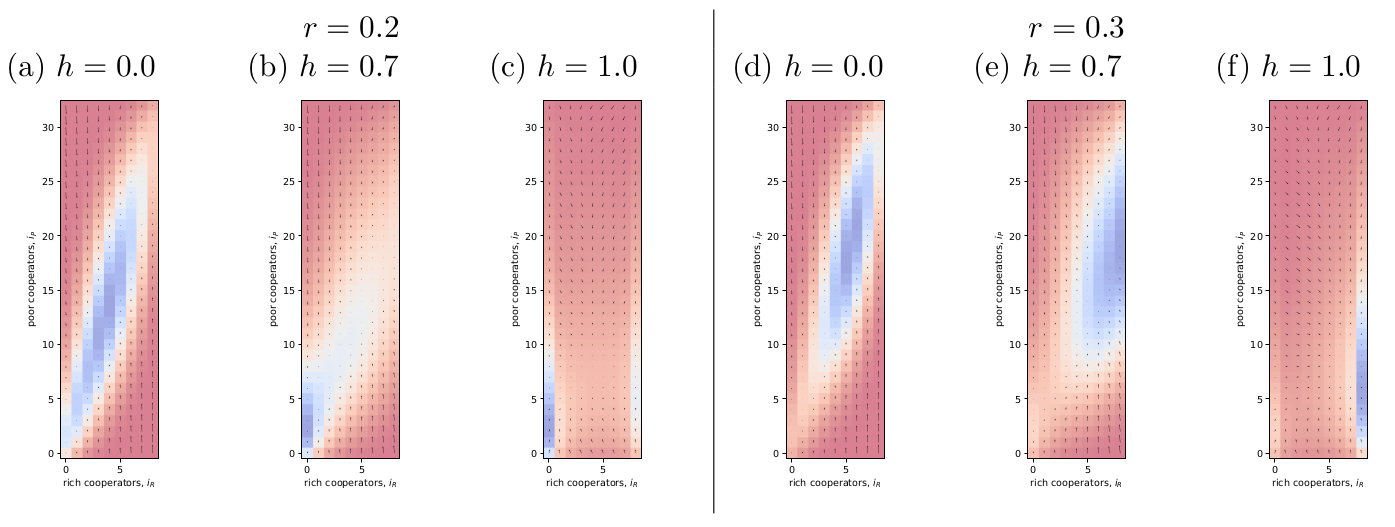
Figure 1: Try to replicate Fig. 2 of Vasconcelos et al. (2014). I chose a smaller population size to speed up the calculations, but I’m getting qualitative agreement with their results.
The process clarified a few points for me:
- The transition probabilities in Eq. \ref{T_k} are for a switch in strategy only, i.e. \(X \neq Y\).
- Therefore, \(\mu\) does not need to be scaled in Eq. \ref{T_k}; it is properly the chance that the candidate will flip to a different strategy, and there is only 1 different strategy.
- Poor tend to copy rich, and that’s central to the dynamics (below).
Something that’s interesting about the paper is that they chose parameter values so that, all else being equal, rich would always be doing better than poor. The poor endowment is 0.625 and rich is 2.25. With a met threshold, rich cooperators would have payoff 2.25 while poor defectors much less at 0.625. The consequence is that, no matter what else is happening, poor will be trying to copy rich. It manifests as a strong tendency for poor to move towards the diagonal. Homophily’s effect is to weaken that and make the attractor more circular (figures below).
Something else I noticed: if you look carefully at Fig. 1f, you’ll see that the stationary distribution does not precisely coincide with the apparent attractor in the gradient field. You can see a similar thing in Fig. 2b in the original paper. There are two things going on here. First, a small vector does not mean that the dynamics has a tendency to stay in that position. Two large probabilities in opposite directions (e.g., chance to gain and to lose a poor cooperator) will cancel out. Second, when \(h \rightarrow 1\), the edges of the graph, in addition to the corners, become sticky. When \(h=1\), the there are no cooperators or no defectors in a wealth class, then the dynamics cannot leave the edge until a mutation occurs.
The stickiness of the edges may partly explain why homophily has the dampening effect on group achievement (Fig. 1 of Vasconcelos et al. (2014)): the dynamics get stuck on a non-cooperative edge and so full cooperation is difficult to achieve. It also might explain why obstinate cooperators help (Fig. 3 of Vasconcelos et al. (2014)): by disallowing zero cooperators, it keeps the dynamics away from the sticky edges under homophily.
To check these ideas, I increased \(\mu\) to triple its original amount and replotted (Fig. 2). It seems that I was right; the stationary distribution stays roughly in the middle of the parameter space, though homophily’s effect can still be seen by the attractive edges.
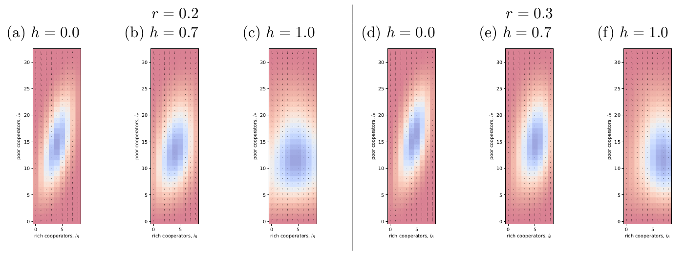
Figure 2: Same as Fig. 1 but I have tripled ‘mu’ to ‘mu = 3/Z’. The idea was to check if sticky edges were the reason for homophily’s effect in their Fig. 1.
I was curious to see how homophily changes things at high risk (Fig. 3). It looks like homophily, which removes copying of rich by poor, causes poor to settle at a lower level of cooperation. I suppose rich have more to lose so they’re more inclined to cooperate.
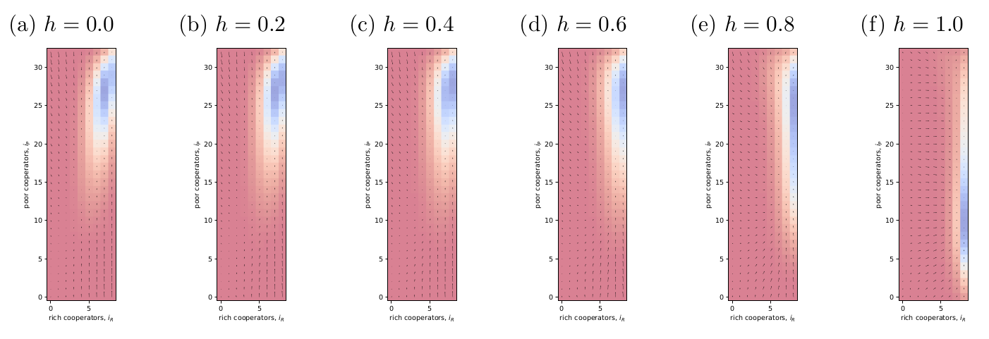
Figure 3: Same as Fig. 1 but I have set risk high ‘r=0.9’ and I’m looking at how varying homophily affects the dynamics.
References
Sigmund, K., De Silva, H., Traulsen, A. and Hauert, C. (2010). Social learning promotes institutions for governing the commons, Nature 466(7308): 861.
Vasconcelos, V. V., Santos, F. C., Pacheco, J. M. and Levin, S. A. (2014). Climate policies under wealth inequality, Proceedings of the National Academy of Sciences 111(6): 2212–2216.