Extinction of undiscovered butterflies + tutorial
Meryl Theng just had a new paper published in Biological Conservation, where she estimated that 46% of Singapore’s butterfly species have been extirpated since 1854. The special thing about this estimate is that it includes all species that existed, including species that went extinct before we had a chance to discover them.
The trick to estimating undiscovered extinctions is the SEUX model. There is a nice write-up about the paper on Ryan’s blog. The paper has also received a good response in the press - The Straits Times and The Star have covered it - and it is generating some interest on Twitter as well.
Rather than add to all of this, I thought this would be a good opportunity to do a short tutorial, so you can use the same method on your own data. We have created an R package, which you can get from the from the SEUX R package repo.
The first step is to install the package, which I have located at ../seux.
install.packages("../seux", repos = NULL, type="source")
library("seux")
Now you should be able to access all of the functions in the package listed below
lsf.str("package:seux")

central_hyper_midP : function (U0, S0, S1, U1, d0)
check_frst_last_detns : function (frstDetn, lastDetn) #... etc.
In this example, we will work with the Singapore birds historical record from Chisholm et al. (2016), which you can download here. So we’ll read that data in:
fName <- "example_data/AppendixS5birdspecieslistSingapore.csv"
raw_data <- read.csv(fName,header=T)
head(raw_data)
We see that this database contains a list of bird species, the year in which they were first recorded, and the year in which they were last recorded

The SEUX model needs the first and last detections, so we’ll make a note of where they are. We can use either the column number or the column header.
frst_col <- 3
last_col <- "Last record"
Then we feed this into the SEUX model.
The usual workflow steps are:
- The
detection_recordof first and last detections of each species is read from a.csv; - The
model_inputs, which is a timeseries of \(S\) (detected extant) and \(E\) (detected extinct), is created from thedetection_record; - Confidence intervals and estimates for the unknown \(U\) (undetected extant) and \(X\) (undetected extinct) can be obtained using the central hypergeometric SEUX model;
- Estimates using the method published in Chisholm et al. (2016) can also be obtained.
detection_record <- get_first_last_detections_from_csv(fName, frst_col, last_col) # 1
model_inputs <- get_model_inputs( detection_record$frstDetn, detection_record$lastDetn) # 2
CIs_estimates <- get_CI_estimate( model_inputs$S, model_inputs$E) # 3
old_estimates <- get_old_estimate( model_inputs$S, model_inputs$E ) # 4
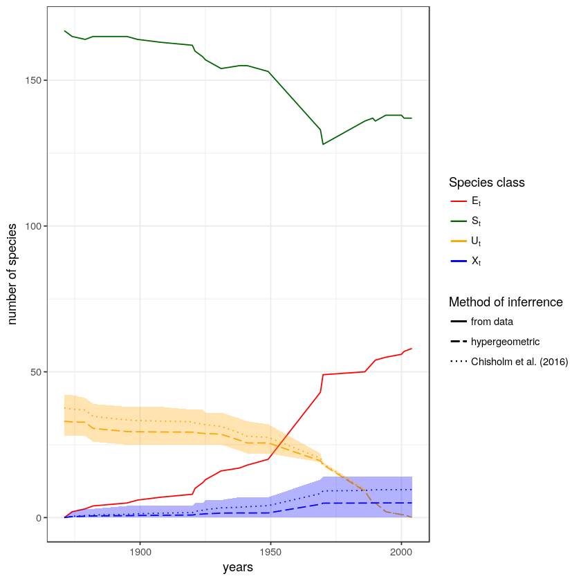
df <- cbind(model_inputs, CIs_estimates, old_estimates)The outputs from the models can be plotted using something similar to this:
library(ggplot2)

plot_output <- function(df) {

    p <- ggplot(df) +
     geom_line(aes(year, S,      color="S", linetype="data")) +
     geom_line(aes(year, E,      color="E", linetype="data")) +
     geom_line(aes(year, U_mean, color="U", linetype="hyper")) +
     geom_line(aes(year, U_old,  color="U", linetype="old")) +
     geom_line(aes(year, X_mean, color="X", linetype="hyper")) +
     geom_line(aes(year, X_old,  color="X", linetype="old")) +
     scale_color_manual(name="Species class",
                       values=c(
                                "S"     = "darkgreen",
                                "E"     = "red",
                                "U"     = "orange",
                                "X"     = "blue"
                                ),
                       labels=c(
                                "S"     = expression(S[t]),
                                "E"     = expression(E[t]),
                                "U"     = expression(U[t]),
                                "X"     = expression(X[t])
                                )
                       ) +
     scale_linetype_manual(name="Method of inferrence",
                       values=c(
                                "data"  = "solid",
                                "hyper" = "longdash",
                                "old"   = "dotted"
                                ),
                       labels=c(
                                "data"  = "from data",
                                "hyper" = "hypergeometric",
                                "old"   = "Chisholm et al. (2016)"
                                )
                       ) +
     geom_ribbon(aes(x=year, ymin=X_lo, ymax=X_hi), fill="blue", alpha="0.3") +
     geom_ribbon(aes(x=year, ymin=U_lo, ymax=U_hi), fill="orange", alpha="0.3") +
     xlab('years') +
     ylab('number of species') +
     theme_bw()

    return(p)

    }

the_plot <- plot_output(df)
print(the_plot)
Here is a plot of the SEUX results above. The yellow line \(U_t\) is the inferred number of undiscovered species over time, and the blue line \(X_t\) is the number of species that went extinct before we had a chance to discover them.
And that’s it!
Of course, the result above is the ‘default’ result that can be obtained using the package. If you would like to do a more in-depth analysis, including exploring the effect of unequal extinction rates for discovered and undiscovered species, the further examples in the Tutorial will guide you.
As always, I’d love to hear from anyone who plans to use the package; just drop me an email. The package is in development, so I’d also welcome any feedback you have about its use or the supporting documentation.
Reference:
Theng M., W. F. A. Jusoh, A. Jain, B. Huertas, D. J. X. Tan, H. Z. Tan, N. P. Kristensen, R. Meier, Ryan A. Chisholm. (2020) A comprehensive assessment of diversity loss in a well-documented tropical insect fauna: Almost half of Singapore’s butterfly species extirpated in 160 years. Biological Conservation, 242:108401