Playing with a new model for fugitive coexistence
I recently read a paper by Kawecki (2017), which presents a new mechanism for something analogous to fugitive coexistence. The paper has a really great literature overview, which I won’t be able to do justice here. In short, fugitive coexistence is when an inferior species persists on a patchy landscape by being a better coloniser: when a local extinction occurs, they are quicker to arrive at the patch and so exploit the time window before the superior competitor arrives. But Kawecki had another idea about how coexistence could occur.
In the paper, Kawecki explores the coexistence of a ‘jack of all trades’ - who has the same fitness in every patch thanks to phenotypic plasticity - with an adaptable species - who relies upon (slow) genetic evolution to become the superior species in the local patch. Similar to fugitive coexistence above, the plastic species can also persist by exploiting a time window, but not because they are faster colonisers. Instead, the time window is provided by the time that it takes for the adaptable species to become locally adapted to the patch.
The relative fitness of the plastic species is constant, but includes a cost of plasticity \(c\)
\[w_{P} = e^{-c}\]The fitness of the adaptive species on patch \(i\) is a Gaussian relationship measuring how well its trait \(x\) matches the optimal value in the patch \(\xi_i\)
\[f_i(x) = e^{ -s (x - \xi_i)^2 }\]where \(s\) is the selection strength.
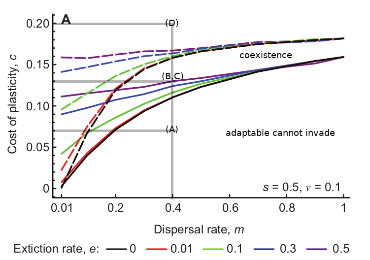
Figure 1 from the paper (reproduced below) explores the invasion success of each type into a population dominated by the other. Between the solid and dashed lines is the sweet spot in parameter space where the plastic and the adaptable species can coexist.

Solid lines: minimum cost of plasticity that allows the adaptable species to invade. Dashed lines: maximum cost of plasticity that allows the plastic species to invade. Between the lines: species can coexist. Grey lines: location in parameter space of my simulation examples (below).
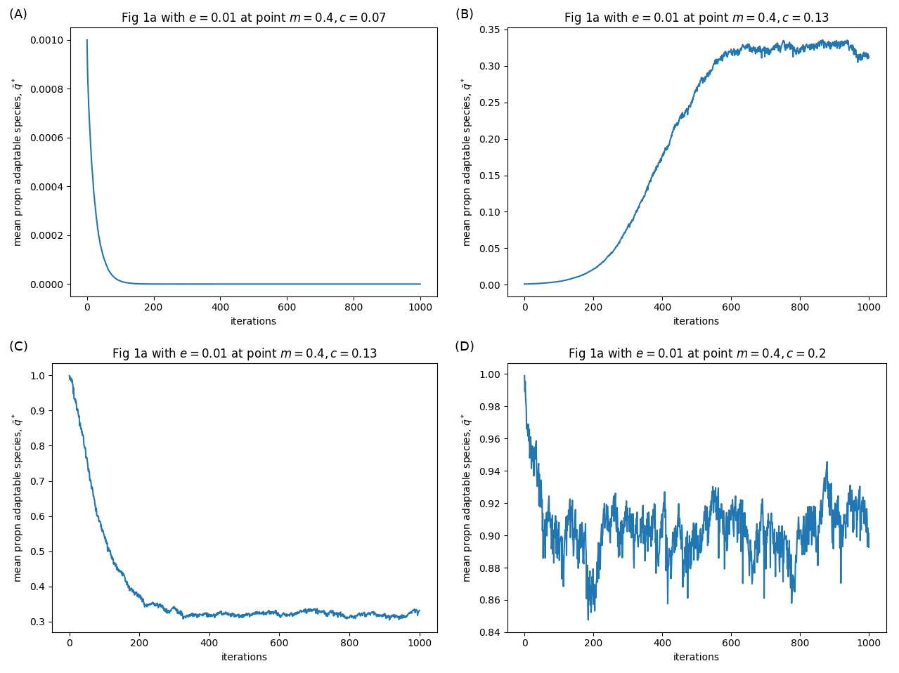
I was interested in implementing the simulations, so I wrote some Python code to track the mean proportion of adaptable type \(\bar{q}^*\) in time for the parameter values I indicate with grey lines above. My results are shown in the figure below.

Results from my simulations. Panel labels correspond to labels in the figure above.
When the cost of plasticity \(c\) is low (\(c=0.7\)), and a small number of adaptable species are introduced to a population of plastics, the adaptables cannot invade the system (panel A). When the cost of plasticity \(c\) is higher (\(c=0.13\)), the adaptable species can invade, and the system equilibriates around 32% adaptable, 68% plastic (B). Similarly, a small number of plastic species introduced to a population of adaptables can invade, and seems to equilibriate at the same 32 vs 65% ratio (C). Interestingly, I found that the plastic species seemed to persist above the dashed lines (e.g. \(c=0.2\)) at very low densities, i.e. below the 0.1 cut-off that was used as a criterion for invasion success (D). I wonder what that means?
Notes on the implementation:
- Python scripts can be downloaded from here: kawecki-2017-fugitive-coexistence on GitHub
- What is called \(e\) in the text appears to be also called \(p\) in the equations.
- For Equation 6 I used: \(x_i^* = \ldots = x_i + 2sv(\xi_i - x_i)\)
- For Equation 7 I replaced the \(1-q\) in the numerator with \(1-p\). It’s the number of other patches from which immigrants can arrive, which is depending on the patch-extinction rate.
- For Equation 7 and 2 in the simulations, I used the proportion of patches that survived directly rather than \(1-p\).
- For Equation A1 I got: \(x_i' = (1-m) \left( (1-2sv) x_i + 2sv \xi_i \right) + m \bar{x}^*\)
Reference:
Kawecki, T.J., 2017. Fugitive coexistence mediated by evolutionary lag in local adaptation in metapopulations. Annales Zoologici Fennici 54(1-4):139-153.