Stochastic evolutionary dynamics of the Volunteers' Dilemma
The purpose of this blog post is to use a recent paper by Tutić (2021) to teach myself about stochastic evolutionary game theory.
Tutić’s (2021) model concerns the Volunteer’s Dilemma, which is a public goods game where the public good is provided if at least one group member cooperates. In the replicator dynamics, cooperators can always invade a population of defectors. However, as the group size increases, the proportion of cooperators in the population at the evolutionary steady-state declines (see Tutić (2021) Fig. 6), which increases the risk that cooperators will be lost from a finite population where stochastic forces are strong.
The game payoffs to defectors are 0 if no other group members are cooperators (no public good produced), and \(\beta\) if there is at least one. The payoff to cooperators is always \(\beta - \gamma\), where \(\gamma\) is the cost of providing the public good. Tutić (2021) used the default values of \(\beta = 4\) and \(\gamma = 2\).
The contribution of the game to fitness is governed by selection strength \(w\), so the fitness of cooperators and defectors is
\[\begin{align} \pi^w_c(i, h) &= 1 - w + w \pi_c(i, h), \\ \pi^w_d(i, h) &= 1 - w + w \pi_d(i, h), \end{align}\]where \(\pi_x(i, h)\) are the expected payoffs in a population (size \(n\)) with \(i\) cooperators from games with \(h\) players. They are,
\[\begin{align} \pi_c(i, h) &= \beta - \gamma, \\ \pi_d(i, h) &= \beta \left( 1 - \frac{ {n-i-1 \choose h-1} }{ {n-1 \choose h-1} } \right). \end{align}\]The combinatorial term is the probability that all other members of the defector’s group are defectors, which has a hypergeometric distribution.
The dynamics are modelled as a Moran process, and we’re interested in the transitions in the number of cooperators \(i\). The probability of a transition from \(i\) cooperators to \(i+1\) is
\[\begin{equation} p_{i, i+1} = \left( \frac{n-i}{n} \right) \left( \frac{\pi^w_c(i,h) i}{\pi^w_c(i,h) i + \pi^w_d(i,h)(n-i)} \right), \end{equation}\]where the first bracketed term is the probability that a defector dies, and the second term is the probability that they are replaced by a cooperator, which depends on the average fitness of cooperators above. By similar reasoning,
\[\begin{equation} p_{i, i-1} = \left( \frac{i}{n} \right) \left( \frac{\pi^w_d(i,h) i}{\pi^w_c(i,h) i + \pi^w_d(i,h)(n-i)} \right), \end{equation}\]and \(p_{i, i} = 1 - p_{i, i+1} - p_{i, i-1}\).
Tutić (2021) used the method of Nowak (2006) to find the cooperator fixation probabilities. There seems to be a typo in the second equation on page 7 (the `\(\ldots\)’); according to page 99 of Nowak (2006), the fixation probability given initial \(i\) should read
\[\begin{equation} x_i = x_1 \left( 1 + \sum_{j=1}^{i-1} \prod_{k=1}^j \frac{\pi_d^w(k,h)}{\pi_c^w(k,h)} \right). \end{equation}\]To find cooperator fixation probabilities, I decided instead to use the general Markov approach. Warren Weckesser at Colgate University has made available some nice lecture notes, but note that my transition matrix \(P\) is the transpose of what Weckesser uses, to match the convention used in some other references below.
Define the transition matrix \(P(i,j) = p_{i,j}\), which is the probability that the population will transition from \(i\) to \(j\) cooperators. Reorder the transition matrix into its canonical form,
\[\begin{equation} P = \begin{bmatrix} I & \mathbf{0} \\ R & Q \\ \end{bmatrix}, \end{equation}\]where, in our case, \(I\) is a \(2 \times 2\) matrix corresponding to the absorbing states \(i=0\) and \(i=n\). The fundamental matrix
\[\begin{equation} N = (I - Q)^{-1}. \end{equation}\]The \(i\)th row \(NR\) gives the probabilities of ending up in each of the absorbing states (columns) given that the process started in the \(i\)th transient state. My Fig. 1 below matches Tutić’s (2021) Fig. 2 and 5.

Tutić (2021) used simulations to explore the long-term dynamical behaviour. Tutić (2021) reports that, when \(h=5\), most simulations went to fixation unless the selection was strong, e.g., \(w=0.8\).
\(N(i, j)\) gives the expected number of times that the process is in the \(j\)th transient state given that it started in the \(i\)th transient state. Therefore, the sum of the \(i\)th row of \(N\) gives the expected number of times that the process will be in some transient state given that the process started in the \(i\)th transient state.
Fig. 2 shows the expected transient times I found using \(N\) when \(h=5\) and \(w=0.8\) for different initial values of \(i\). For most initial values, the transient time is quite long, as Tutić (2021) reports.

When an absorbing Markov chain spends a long time in transient states, the quasi-stationary behaviour can be characterised using the methods reviewed in van Doorn and Pollett (2013) and used in e.g., Day and Possingham’s (1995) paper about metapopulation persistence. Following Day and Possingham (1995), the left eigenvector corresponding to the maximal eigenvalue \(\mu_1\) of \(Q\) gives the quasi-stationary distribution. \(\mu_1\) is always less than 1, and the closer \(\mu_1\) is to 1, the longer the process continues before absorption. Van Doorn and Pollett (2013) defines the spectral gap \(\gamma\) as the distance between the two largest eigenvalues, and if \(\gamma\) is is substantially larger than the decay parameter \(\alpha = 1-\mu_1\), then the dynamics will exhibit quasi stationary behaviour, i.e., relatively fast convergence to the limiting conditional distribution, and eventual evanescence after a much longer time.
Fig. 3 shows the quasi-stationary distribution found from the leading left eigenvector of \(Q\). The expected value matches the expected value Tutić (2021) observed in simulations (compare with Fig. 6 in Tutić (2021)). The systems spends most of its time near the all-defector state, which puts it at risk of eventually losing the cooperators from the population.
I found \(\mu_1 = 0.9999989\), which is close to 1 and indicates the transient dynamics will continue a long time before fixation. I found \(\gamma = 5.5 \times 10^{-3}\) and \(\alpha = 1 \times 10^{-6}\), which indicates quasi-stationary behaviour.

The model assumes that, if there is more than one cooperator in the group, then they will all pay the cost \(\gamma\) to provide the public good. I wondered, what would happen if only one cooperator provided the good, e.g., if they draw straws or one is randomly chosen to do the job first, or if they split the costs between them?
I modified the cooperator payoff
\[\begin{equation} \pi_c(i, h) = \beta - \sum_{k=0}^{h-1} \frac{\gamma}{k+1} \cdot \frac{ {i-1 \choose k} {n-i \choose h-1-k} }{ {n-1 \choose h-1} }, \end{equation}\]where the sum is over the number of other group members that are cooperators \(k\), the first fraction represents the cost of providing the good given that \(k\), and the second fraction represents the probability of being grouped with \(k\) other cooperators (hypergeometric distribution again).
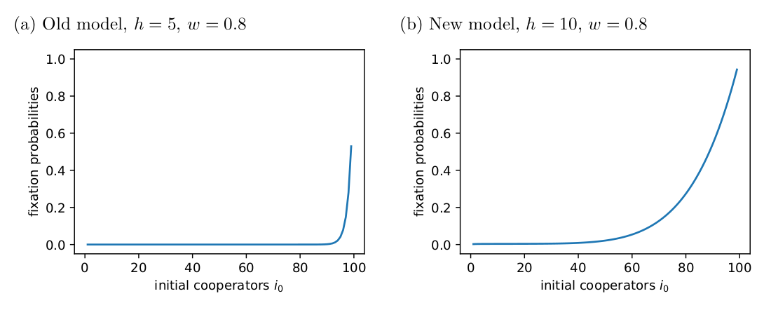
In the new model, group size still has a negative effect on fixation probabilities, but it is less severe than in the original model and doesn’t have such strong effects when the intial number of cooperators is high (Fig. 4).

A population with an initially modest number of cooperators is now more likely to go to the all-cooperator absorbing state (Fig. 5).
However, the quasi-stationary distribution still spends most of its time near the all-defect absorbing state (Fig. 6). Therefore, while there is a better chance in the new model that the population will be absorbed to the all-cooperator state, the overall story that the original Tutić (2021) model tells is still true: cooperation becomes harder to maintain as group size increases.

The code I used for this blog post is available on Github: tutic-2021-playground.
References
Day, J. R. and Possingham, H. P. (1995). A stochastic metapopulation model with variability in patch size and position, Theoretical Population Biology 48(3): 333–360.
Nowak, M. A. (2006). Evolutionary dynamics: exploring the equations of life, Harvard University Press.
Tutić, A. (2021). Stochastic evolutionary dynamics in the volunteer’s dilemma, The Journal of Mathematical Sociology: 1–20.
van Doorn, E. A. and Pollett, P. K. (2013). Quasi-stationary distributions for discrete-state models, European Journal of Operational Research 230(1): 1–14.