Transient dynamics in neutral models
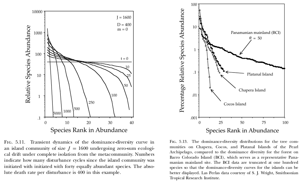
In their 10-year-anniversary review of neutral theory (Hubbell, 2001), Rosindell et al. (2011) note that little work has been done on the model’s transient dynamics. Transient dynamics are nonetheless interesting because they can capture important processes occurring in recently disturbed landscapes. For example, if forest is cleared such that only a small patch remains, then the number of species in that patch will continue to decline over time (i.e. extinction debt). As another example (Hubbell, 2001, p. 140–142), the Pearl Archipelago in the Bay of Panama was once a continuous coastal plain attached to the mainland. As the water rose since the last glacial maximum, the land became separated into a series of islands. Therefore, the species abundance curves on those islands may carry the signature of their mainland connection along with their current size and distance to the mainland (comparing his Fig. 5.11 and 5.13; see also Sin et al. 2022).
The Rosindell et al. (2011) paper was almost 10 years ago, so I wondered what work had been done on transient neutral dynamics since then. Missa et al. (2016) provide a more recent review of the literature, and they state that it remains the case that nearly all analytical predictions from the neutral model are for dynamic equilibrium. The reason for this is obviously because the mathematics of transient dynamics is tricky.
One route to simplifying the mathematics is to relax the zero-sum assumption. By treating each species and its transitions between abundance states as independent from other species, Chisholm (2011), for example, obtained the species abundance distributions in time and the time taken to equilibrium. Fung et al. (2020) notes that this non-zero-sum approximation may be justified if the abundance of a species is nearly always small relative to the community abundance. I gather that Vallade et al. (2003) was the first to use this kind of approach; they made the independent-species assumption to find the steady-state species abundance distributions in both the metacommunity and local community.
Relaxing the zero-sum assumption generally leads to a system of ordinary differential equations. For example, Wu et al. (2020) recently gave the following system of equations

where each \(p_j\) is the probability that an independent species has abundance \(j\) at time \(t\). This system of equations can be numerically integrated in the usual way (see code snippet below), which Wu et al. (2020) used to explore immigration, emigration, and the effect of the initial species abundance distribution.
i0 = m = rep(0,1,N+1) # initialise vector p with all zeros
i0[p0+1] = 1 # initialise so that there is 1 species with abundance j, p_j = 1
w = i0
t = 0
while(t<tp) {
for(s in 1:(N+1)) { # all the states including 0
# each of these cases are a row in Eq. 2.1 such that p_j(t+1) = p_j(t) + dp_j(t) / dt
# or Eq. 2.3 for the coefficients is a bit easier to read
if(s==1) { # p0
# p_0(t+1) = p_0(t) + dt ( p_1(t) - v p_0(t) )
m[s]=(w[s+1]-v*w[s])*dt+w[s]
}else if(s==2) { # p1
# p_1(t+1) = p_1(t) + dt ( v p_0(t) - (2-u) p_1(t) + 2 p_2(t)
m[s]=(v*w[s-1]+2*w[s+1]-(2-u)*w[s])*dt+w[s]
}else if(s>2 & s<N+1) { # p(s-1)
# p_i(t+1) = p_i(t) + (i-2) (1-u) p_{i-... etc.
m[s]=((s-2)*(1-u)*w[s-1]+s*w[s+1]-(s-1)*(2-u)*w[s])*dt+w[s]
}else if(s==N+1) { #last state
m[s]=((s-2)*(1-u)*w[s-1]-(s-1)*w[s])*dt+w[s]
}
}#s
w = m # update w
t = t + dt # update time
}Another way to simplify the situation is to assume that the community is large and use a continuous approximation. McKane et al. (2004) started with the one-step transition probabilities turned them into a continuous derivative. The provides the master equation with some technicalities on the boundaries. An impediment to solving the time-dependence is that the transition probabilities are non-linear functions of the number of individuals of each species \(j\) in the community, \(N_j\). However, they can get an approximation by assuming that the total number of individuals is large. In that case, they can assume that \(P(N_j , t)\) is roughly Gaussian, and the motion of its peak is treated deterministically. Then they find a deterministic equation for the motion of this peak and the width of its distribution. Relatedly, Azaele et al. (2006) (also explained in Azaele et al. (2016)) also used a continuous approximation combined with a Taylor expansion to obtain the dynamics of the species abundance distributions near the steady state.
There are a few special cases in which analytic transient dynamics can be obtained. Halley and Iwasa (2011) considered a neutral community with no immigration and no speciation, so the system will equilibriate at a single species. They chose an initial condition equivalent to the broken stick model (equivalent to assuming that every species-abundance distribution is equally probable), and were able to obtain a relatively simple expression for species richness in time (their Eq. 5).
Another way to make progress on the transient dynamics is to focus on the dynamics of diversity indices instead. By modelling space as a network of patches and permitting speciation, the temporal dynamics of Simpson’s Index and its multi-patch analogues can be solved with numerical integration of a relatively low-dimensional system of ODEs (Vanpeteghem and Haegeman, 2010). This built on an earlier paper, which found dynamical equations for the Simpson diversity index for a local community (Vanpeteghem et al., 2008). The trick is to obtain (exact) dynamical moment equations from the master equation, and then use the first few moements to compute mean and variance of diversity indices.
It’s worth an aside to talk about the Simpson’s Index, as Vanpeteghem et al. (2008) notes, it had been known for a while that Simpson diversity is “somehow compatible” with neutral theory. He and Hu (2005) explicitly derived the relationship between Simpson’s diversity \(D\) and Hubbell’s fundamental biodiversity number \(\theta\) as
\[D = \frac{\theta}{1+\theta}.\]They achieved this by obtaining a continuous form of the expression for the relative species abundance curve from neutral theory and integrating it. Perhaps more directly, Etienne (2005) observed that the sequential construction scheme used to obtain a sample of J individuals from a metacommunity (the algorithm Hubbell (2001) gives in Fig. 9.1) immediately implies that the probability that the first two individuals drawn are the same species — the definition of Simpson’s diversity — is the expression above; though that does raise the question of where the scheme comes from in the first place (see later post for update).
Why do transient dynamics matter? One might be interested in transient dynamics in and of themselves, such as the forest clearing or sea-level change examples I began with. However, transients also matter if one can’t be sure that the system being studied – or the metric of interest – is at dynamical equilibrium. Using simulations, Missa et al. (2016) observed that community patterns reach equilibrium in approximately the following order: species richness, species abundance rank, species abundance distribution, phylogenetic structure. As another example, the empirically observed lognormal-like relative species abundance curves (i.e. with a high central mode) only occur in highly dispersal-limited communities in the transient dynamics; however, when the migration rate is very low, it takes a long time for the dynamical equilibrium to be reached anyway, so this might be their usual state (Chisholm and Burgman, 2004). As a final example, Tittensor and Worm (2016) used spatially explicit simulations to explore how neutral theory might explain the latitudinal biodiversity gradient. They found that, when turnover and speciation rates were temperature dependent, the latitudinal gradient appeared– but only in the transient dynamics.
References
Azaele, S., Pigolotti, S., Banavar, J. R. and Maritan, A. (2006). Dynamical evolution of ecosystems, Nature 444(7121): 926–928.
Azaele, S., Suweis, S., Grilli, J., Volkov, I., Banavar, J. R. and Maritan, A. (2016). Statistical mechanics of ecological systems: Neutral theory and beyond, Reviews of Modern Physics 88(3): 035003.
Chisholm, R. A. (2011). Time-dependent solutions of the spatially implicit neutral model of biodiversity, Theoretical Population Biology 80(2): 71–79.
Chisholm, R. A. and Burgman, M. A. (2004). The unified neutral theory of biodiversity and biogeography: comment, Ecology 85(11): 3172–3174.
Etienne, R. S. (2005). A new sampling formula for neutral biodiversity, Ecology Letters 8(3): 253–260.
Fung, T., Verma, S. and Chisholm, R. A. (2020). Probability distributions of extinction times, species richness, and immigration and extinction rates in neutral ecological models, Journal of Theoretical Biology 485: 110051.
Halley, J. M. and Iwasa, Y. (2011). Neutral theory as a predictor of avifaunal extinctions after habitat loss, Proceedings of the National Academy of Sciences 108(6): 2316–2321.
He, F. and Hu, X.-S. (2005). Hubbell’s fundamental biodiversity parameter and the simpson diversity index, Ecology Letters 8(4): 386–390.
Hubbell, S. P. (2001). The unified neutral theory of biodiversity and biogeography, Vol. 32, Princeton University Press, Princeton, USA.
McKane, A. J., Alonso, D. and Solé, R. V. (2004). Analytic solution of Hubbell’s model of local community dynamics, Theoretical Population Biology 65(1): 67–73.
Missa, O., Dytham, C. and Morlon, H. (2016). Understanding how biodiversity unfolds through time under neutral theory, Philosophical Transactions of the Royal Society B: Biological Sciences 371(1691): 20150226.
Rosindell, J., Hubbell, S. P. and Etienne, R. S. (2011). The unified neutral theory of biodiversity and biogeography at age ten, Trends in Ecology & Evolution 26(7): 340–348.
Tittensor, D. P. and Worm, B. (2016). A neutral-metabolic theory of latitudinal biodiversity, Global Ecology and Biogeography 25(6): 630–641.
Vallade, M., and Houchmandzadeh, B. (2003). Analytical solution of a neutral model of biodiversity, Physical Review E 68(6): 061902.
Vanpeteghem, D. and Haegeman, B. (2010). An analytical approach to spatio-temporal dynamics of neutral community models, Journal of Mathematical Biology 61(3): 323–357.
Vanpeteghem, D., Zemb, O. and Haegeman, B. (2008). Dynamics of neutral biodiversity, Mathematical Biosciences 212(1): 88–98.
Wu, Y., Chen, Y., Chang, S.-C., Chen, Y.-F. and Shen, T.-J. (2020). Extinction debt in local habitats: quantifying the roles of random drift, immigration and emigration, Royal Society Open Science 7(1): 191039.