The method of confidence belts illustrated
What is a confidence interval, really? We all learnt in undergrad how to find CIs for a standard distribution, but plugging numbers into equations never gave me a deep intuition for what was really going on.
A worded definition is probably more helpful. Paraphrasing a bit from Wikipedia, we can think of the meaning of the confidence interval in terms of the procedure that we used to construct it.
If this procedure for constructing confidence intervals is repeated on many samples, then the fraction of times that the true parameter value will fall within the different intervals will approach \(\gamma\).
So how does this meaning get translated into a procedure?
The classic reference for CIs is Neyman (1937), but the language is a bit antiquated. Instead, I recently found a paper by Feldman & Cousins (1998), which presented the idea in a very effective way. Note that this paper swaps the notation of \(\alpha\) and \(\gamma\) from their most common usage, so I have swapped it back for this blog post.
The key is their Fig. 1, reproduced below. The figure concerns some outcome \(x\) whose value probabilistically depends on a parameter \(\mu\). In the figure, we see many horizontal lines. Each line represents an interval over the \(x\) values, and it has been been specifically constructed so that it possesses a special property: for that value of \(\mu\), there is a probability \(\gamma\) that \(x\) will take a value somewhere on that line, i.e. \([x_1, x_2]\) such that \(P(x \in [x_1, x_2] \mid \mu ) = \gamma\). These horizontal lines are called acceptance intervals.
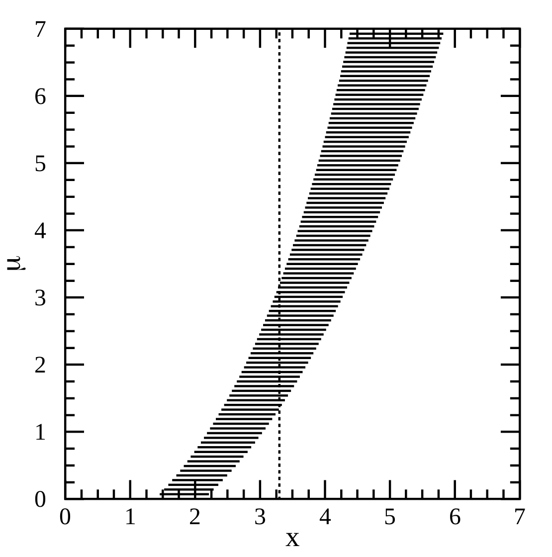
In the figure, they have also drawn a vertical dotted line. The vertical line corresponds to a particular observation of \(x\) from some sample or experiment; in this case, \(x \approx 3.26\). Where this vertical line crosses over the horizontal lines gives us the confidence interval. The confidence interval \([\mu_1, \mu_2]\) is the union of all values \(\mu\) for which the observed \(x\) falls within \(\mu\)’s acceptance interval.
So this procedure matches our worded definition above. If we use this procedure to construct confidence intervals, then we know for sure that - over many repeated samples - the true parameter value will fall within the confidence intervals a \(\gamma\) fraction of times. We know this because that’s how we specifically constructed our acceptance intervals, by making sure that every horizontal line has \(P(x \in [x_1, x_2] \mid \mu ) = \gamma\) for whatever values that \(\mu\) might take.
This way of thinking also clarifies to my mind why there are different methods for obtaining confidence intervals, and why there are questions about the best way of doing so. If the only thing required of the acceptance interval is \(P(x \in [x_1, x_2] \mid \mu ) = \gamma\), then I could do all kinds of wild things. I could push all of the horizontal lines as far to the left as they can go. Or I could put gaps in the lines so that they are not intervals at all, and call them acceptance sets. Then the confidence intervals (or sets) that I obtain would still satisfy the meaning of the confidence interval - they’d still contain the true \(\mu\) value in \(\gamma\) proportion of samples - but their properties might not be very intuitively satisfying.
Intuitively, the acceptance intervals should be somehow ‘centred’ in the probability distribution, they should all be positioned relative to one another so that any vertical lines we draw will not have any ‘gaps’ (i.e. our confidence intervals are actual intervals), and we might prefer the resulting confidence intervals to be short. Satisfying these kinds of requirements is the work of the auxiliary criteria, which are basically rules for constructing and positioning the horizontal lines in Fig. 1. Feldman & Cousins (1998) introduce the concept of auxiliary criteria near Eq. 2.5, including the familiar criteria for the two-sided central confidence interval
\[P(x < x_1 \mid \mu) = P(x > x_2 \mid \mu) = \alpha/2.\]They continue on to introduce a clever new auxiliary criteria (add \(x\) values to the acceptance interval in order of decreasing likelihood ratio), which produces confidence intervals with the pleasing property that they automatically switch from one- to two-sided as the small signals that physicists measure become more statistically significant. In a later blog post, I hope to share a different example, which contrasts auxiliary criteria for discrete distributions and compares their performance.
References:
Feldman, G. J. and Cousins, R. D. (1998). Unified approach to the classical statistical analysis of small signals, Physical Review D 57(7): 3873.
Neyman, J. (1937). X – outline of a theory of statistical estimation based on the classical theory of probability, Philosophical Transactions of the Royal Society of London A 236(767): 333–380.