The Principle of Indifference in ecological modelling
(Update April 2019: a paper on the topic below has now been published in MEE)
Qualitative modelling
Qualitative modelling (QM) holds the promise of obtaining predictions from dynamical models even when we don’t have all the data needed to parameterise them. How does QM achieve this? In short, the idea is to explore the range of possible parameter values to create an ensemble of possible predictions, and then interpret those predictions probabilistically and/or qualitatively. For example, if 89% of models predict that rabbit control will increase penguin populations on Macquarie Island, then that might be considered moderate support for that prediction occurring in the real world.
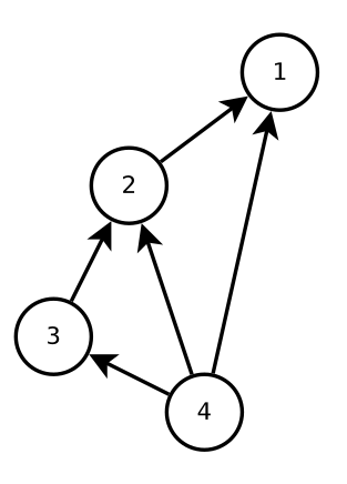
Let’s consider a pest control example in more detail. Imagine that we know which species are in an ecosystem and how they interact (who eats whom, who competes with whom, etc.), and so we have an interaction network like the one below. Species 1 is the pest, and want to predict whether pest-control of species 1 will have a positive or negative effect on species 2, 3, and 4. The difficulty with making this prediction is that there are both direct and indirect effects in the system. So while we might expect that decreasing the number of species 1 will increase the numbers of its prey species 2, the indirect effect through species 3 and 4 might instead lead to a decrease in species 2.
One way to predict the effects of pest control is to model it is a negative press perturbation. This approach makes a number of assumptions (Google: near-equilibrium assumptions), but for the moment, we’ll assume that it is sufficient for our purposes. In order to use this modelling approach, we must quantify the interaction strengths between every pair of species in the network, which are encoded in the community matrix \(A\). For example:
\[A = \begin{pmatrix} -0.522 &+0.733 & 0 &+0.835 \\ -0.632 &-0.013 &+0.113 &+0.428 \\ 0 &-0.223 &-0.193 &+0.001 \\ -0.839 &-0.234 &-0.298 &-0.134 \\ \end{pmatrix}\]Then by analysing \(A\), we can predict whether suppressing species 1 will have a positive or negative effect on the other species in the network.
The challenge with this modelling approach is that it requires a lot of data that we usually don’t have. Usually, we have no idea what the interaction-strength values - the \(a_{i,j}\) values in matrix \(A\) - are. We don’t know anything about them except their sign (positive or negative), and that the model can be scaled so that the values \(0 < \lvert a_{i,j} \rvert < 1\).
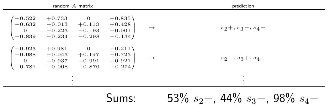
One QM technique for circumventing this problem is to use Monte Carlo sampling (e.g. Raymond et al. 2011). The steps are generally as follows:
- Randomly sample magnitudes for \(a_{i,j}\) from a uniform distribution, to create many \(A\) matrices
- Test plausibility criteria (e.g. the population dynamics must be stable) to each \(A\) matrix and keep only those who pass
- Count the proportion of positive and negative effects predicted by each \(A\) on each species
- The proportion of positive versus negative effects on a species reflect our belief in that outcome
In the hypothetical example below, if we found that 98\% or randomly chosen \(A\) matrices predicted a negative effect on species 4, then we would interpret that as strong evidence that the population of species 4 will decline.
A philosophical interlude
Before continuing, I want to ponder a question: why did we sample \(a_{i,j}\) values from a uniform distribution? There is something very appealing about doing so. If we are completely ignorant of the values of \(a_{i,j}\), then we have no reason to preference any value \(a_{i,j}\) over any other. The uniform distribution expresses this: it treats every possible value of \(a_{i,j}\) as equally likely.
This intuition is the basis of the Principle of Indifference: if we have no reason to distinguish between possible scenarios, then we should favour them equally. The most familiar example might be the roll of a die. There are 6 possible outcomes, and there is nothing to distinguish them from one another. Therefore we favour them equally by assigning the same probability 1/6 to each. This also gives the correct (observed) probabilities for a fair die. We can also apply the Principle of Indifference to a continuous space of outcomes. If we blindfolded a person and had them throw a coin on a wooden floor, then we would assign equal probability to each equal-width plank. By an argument involving reducing the widths of those planks to an infinitesimally small size, we obtain a uniform distribution for the position where the coin lands on the floor.
Now consider another scenario. A jar contains a mix of wine and water. All that we know is that the ratio of wine to water is between \(1/3\) and 3. What is the probability that the ratio of wine to water is less than or equal to 2?
If we apply the uniform prior to the ratio of wine to water, we obtain
\[P \left( \frac{\text{wine}}{\text{water}} \leq 2 \right) = \frac{2-1/3}{3-1/3} = \frac{5}{8}\]However, a perfectly equivalent question is: what is the probability that the ratio of water to wine is greater than 1/2? If we apply the uniform prior to this question, then we obtain
\[P \left( \frac{\text{water}}{\text{wine}} \geq 1/2 \right) = \frac{3-1/2}{3-1/3} = \frac{15}{16}\]which contradicts the answer we got earlier.
Back to ecology
In the hypothetical Monte Carlo simulations above, we randomised over the interaction strengths \(a_{i,j}\) in \(A\); but there are other alternatives:
- The community matrix \(A\) itself is derived from an underlying population-dynamic model, e.g. a Lotka-Volterra model with parameters \(r_i\) and \(b_{i,j}\), so why not randomise over them?
- Species response is the sum of all positive and negative feedbacks, e.g. the `weighted-predictions matrix’ of Dambacher (2003). We could give each feedback equal weight and interpret those proportions as a probability instead?
- Or we could try to incorporate some limited background information. For example, we observe skewed interaction-strength magnitudes in nature (e.g. Neutel et al., 2002), so why not sample \(a_{i,j}\) from a skewed distribution?
All of these seem valid ways to define the model and sample the parameters, however - just like the wine/water paradox - they will give different prediction probabilities.
References
Neutel, A.-M., Heesterbeek, J. A. and de Ruiter, P. C. (2002). Stability in real food webs: weak links in long loops, Science 296(5570): 1120-1123.
Raymond, B., McInnes, J., Dambacher, J. M., Way, S. and Bergstrom, D. M. (2011). Qualitative modelling of invasive species eradication on subantarctic Macquarie Island, Journal of Applied Ecology 48(1): 181-191.