Permanence and the distance from the convex hull to the interior equilibrium
Background
To use permanence, Lotka-Volterra dynamics have to be assumed, because it is only in this case that a sufficient condition for permanence is known:
\[\dot{x}_{i} = x_i \cdot f_i(x) = x_i \cdot (r_i + (A \cdot x)_i) \quad \forall i = 1, \ldots, n.\]Such a dynamical system is permanent if two conditions hold (Hofbauer and Sigmund 1988, The theory of evolution and dynamical systems p. 98).
- It is dissipative; this is true for Lotka-Volterra systems where all the basal species are self-limiting and heterotrophs cannot survive without their prey.
- That: \(P(x) = \prod_i x_{i}^{p_i}\) for some \(p_i>0\) is an average Lyapunov function.
In dissipative Lotka-Volterra systems, the test for permanence reduces to a linear programming problem (Jansen 1987, J. Math. Biol.; Law & Morton 1996, Ecology).
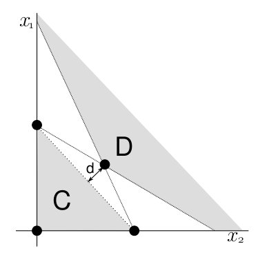
An alternative way of describing the system, pursued in an unpublished paper by Richard Law and R. Daniel Morton, is in terms of the convex hull \(C\) and the set \(D\) where the densities of all species are non-increasing. The convex hull of the boundary equilibria is the smallest convex set of which every boundary equilibrium is a member. If this set is disjoint from \(D\), then the system is permanent. So to test for permanence, one can find a hyperplane passing through the interior equilibrium that has a greater value than that of the hyperplane passing through every boundary equilibrium. One can also measure the ‘strength’ of permanence by \(d\), which is the shortest distance from \(C\) to \(D\), which is always the shortest distance from \(C\) to the interior equilibrium \(\hat{x}\) (Figure 1).
Example
You can download the complete example for Octave from my website: mortongen.m.
Consider the four-species system shown in Figure 2 with the parameter values below, adapted from an unpublished paper by Richard Law and R. Daniel Morton, with:
\[A = \begin{bmatrix} -0.000610 & -0.000207 & -0.052365 & -0.001789 \\ -0.000400 & -0.000139 & -0.001260 & -0.064501 \\ 0.005740 & 0.000033 & 0 & -0.096816 \\ 0.000010 & 0.000151 & 0.000399 & 0 \\ \end{bmatrix}\]and
\[r^{T} = \begin{bmatrix} 0.220737 & 0.164163 & -0.087756 & -0.096189 \end{bmatrix}.\]It has an interior equilibrium point:
\[\hat{x} = \begin{bmatrix} 28.230 & 631.560 & 1.356 & 0.983 \end{bmatrix}\]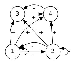
The first step is to find all subsystems \(b = (0,0,0),(1,0,0), \ldots, (1,2,0),(1,3,0),(1,4,0),(2,3,0), \ldots, (2,3,4)\), and then identify which of these have a positive boundary equilibrium \(\hat{x}^{b}\).
If we had all subsystems in subStore, then equilibria would be evaluated by:
for subCnt = 2:noSubs;
	% Acquire list of species absent and present
	present = subStore(subCnt,:);
	present(find(present == 0)) = [];
	absent = 1:nospp; absent(present) = [];

	% Evaluate boundary equilibrium
	ANow = A;
	ANow(absent,:) = []; ANow(:,absent) = [];
	rNow = r; rNow(absent) = [];
	if rank(ANow) == size(ANow,1);
		xSub = ANow-rNow;
% etc.
For our example system, the positive boundary equilibria are:
\[\hat{x}^{(1)} = \begin{bmatrix} 362 & 0 & 0 & 0 \end{bmatrix}\\\] \[\hat{x}^{(2)} = \begin{bmatrix} 0 & 1181 & 0 & 0 \end{bmatrix}\\\] \[\hat{x}^{(1,3)} = \begin{bmatrix} 15.3 & 0 & 4 & 0 \end{bmatrix}\\\] \[\hat{x}^{(2,4)} = \begin{bmatrix} 0 & 637 & 0 & 1.2 \end{bmatrix}\\\] \[\hat{x}^{(1,2,4)} = \begin{bmatrix} 148 & 627 & 0 & 0.3 \end{bmatrix}\]The transversal eigenvalues at the boundary equilibria
\[f(\hat{x}^{}) = r + A\hat{x}^{b}\]are found with code like:
rowofG = A*(xStore(subCnt,:)')+r;and are:
\[f(\hat{x}^{()}) = \begin{bmatrix} 0.22074 & 0.16416 & -0.08776 & -0.09619\ \end{bmatrix}\\\] \[f(\hat{x}^{(1)}) = \begin{bmatrix} 0.00000 & 0.01942 & 1.98934 & -0.09257\ \end{bmatrix}\\\] \[f(\hat{x}^{(2)}) = \begin{bmatrix} -0.02374 & 0.00000 & -0.04878 & 0.08215\ \end{bmatrix}\\\] \[f(\hat{x}^{(1,3)}) = \begin{bmatrix} 0.00000 & 0.15296 & 0.00000 & -0.09443\ \end{bmatrix}\\\] \[f(\hat{x}^{(2,4)}) = \begin{bmatrix} 0.08678 & 0.00000 & -0.18024 & 0.00000\ \end{bmatrix}\\\] \[f(\hat{x}^{(1,2,4)}) = \begin{bmatrix} 0.00000 & 0.00000 & 0.75719 & 0.00000\ \end{bmatrix}\\\]The linear programming problem is then to minimise \(z\) subject to:
\[\begin{align} \sum p_i \cdot f(\hat{x}^{b_1}) + z &\geq 0 \\ \sum p_i \cdot f(\hat{x}^{b_2}) + z &\geq 0 \\ \vdots \\ p_i &\geq 0 \end{align}\]where each positive equilibrium point on the boundary \(\hat{x}^{b_1},\hat{x}^{b_2}, \ldots\) gives rise to a constraint, and \(p_i\) is part of the average Lyapunov function. So if one can find a solution with \(z < 0\), then one can be certain that \(P(x)\) is an average Lyapunov function.
An introduction on how to code linear programming problems in Octave can be found in a previous post. The vector \(p\) for the Lyapunov function, as found using Jansen’s linear program method, is
\[p = \begin{bmatrix} 0.835219 & 1 & 0.077317 & 0.999918 \end{bmatrix}.\]Hofbauer & Sigmund (1988, p. 176-177) states that the convex hull \(C\) can be separated from \(D\) by a hyperplane with a “separating functional” \(pA\), where \(p\) is the same \(p\) used in the Lyapunov function. This separating functional is the vector normal to the hyperplane.
\[\begin{align} \mathbf{n} &= pA \\ &= \begin{bmatrix} -4.5568\times10^{-4} & -1.5835\times10^{-4} & -4.4597\times10^{-2} & -7.3481\times10^{-2} \end{bmatrix} \\ &= \begin{bmatrix} 0.0062014 & 0.0021550 & 0.6069248 & 1 \end{bmatrix}. \end{align}\]The equation for the hyperplane is
\[0 = n_1x_1 + n_2x_2 + n_3x_3 + x_4 + b.\]If one wants to go straight to finding \(d\), then substitute in the boundary steady state for each positive subsystem, reducing the value of \(b\) until the hyperplane is above or equal to every boundary steady state.
So for subsystem \((1)\),
\[\hat{x}^{(1)} = \begin{bmatrix} 361.86393 & 0 & 0 & 0 \end{bmatrix},\]which gives \(b = -2.2441\)
Then subsystem \((2)\) is next, with
\[\hat{x}^{(2)} = \begin{bmatrix} 0 & 1181 & 0 & 0 \end{bmatrix}.\]Substituting into the hyperplane equation gives
\[0.0021550 \times 1181 -2.2441 = 0.30105\]which implies that this boundary steady state is above the hyperplane, therefore it is used to find a revised value of \(b\),
\[b =-2.5451\]This process is continued, checking that all other boundary steady
states are below the plane, and revising \(b\) if they are not, which gives the final value of \(b =-2.5451\).
Now the distance from the interior equilibrium to the plane can be
found. The interior equilibrium is
and so the perpendicular distance from the hyperplane to \(\hat{x}\) is
\[\begin{align} d &= (\mathbf{n}' \hat{x} + b)/|\mathbf{n}| \\ &= \frac{(0.0062014 \times 28.23008 + 0.0021550 \times 631.55967 + 0.6069248 \times 1.35636 + 0.98255 -2.5451)}{1.1698} \\ &= 0.68108, \end{align}\]Alternatively \(d\) can be calculated for each boundary steady state, and the smallest taken as the final value. If xStore stores the values of all the boundary equilibria, then:
d = (n'*xs-xStore(posSubs,:)*n)/norm(n);
disp('d = ')
disp(d)
mind = min(d);
disp('smallest distance = ')
disp(mind)
-
You can download the complete example for Octave from my website: mortongen.m.